Postprocessing and Visualization Updates
COMSOL Multiphysics® version 5.6 brings interactive clipping, partial transparency, and material visualization in plots. Browse all of the postprocessing and visualization updates included in COMSOL Multiphysics® version 5.6 below.
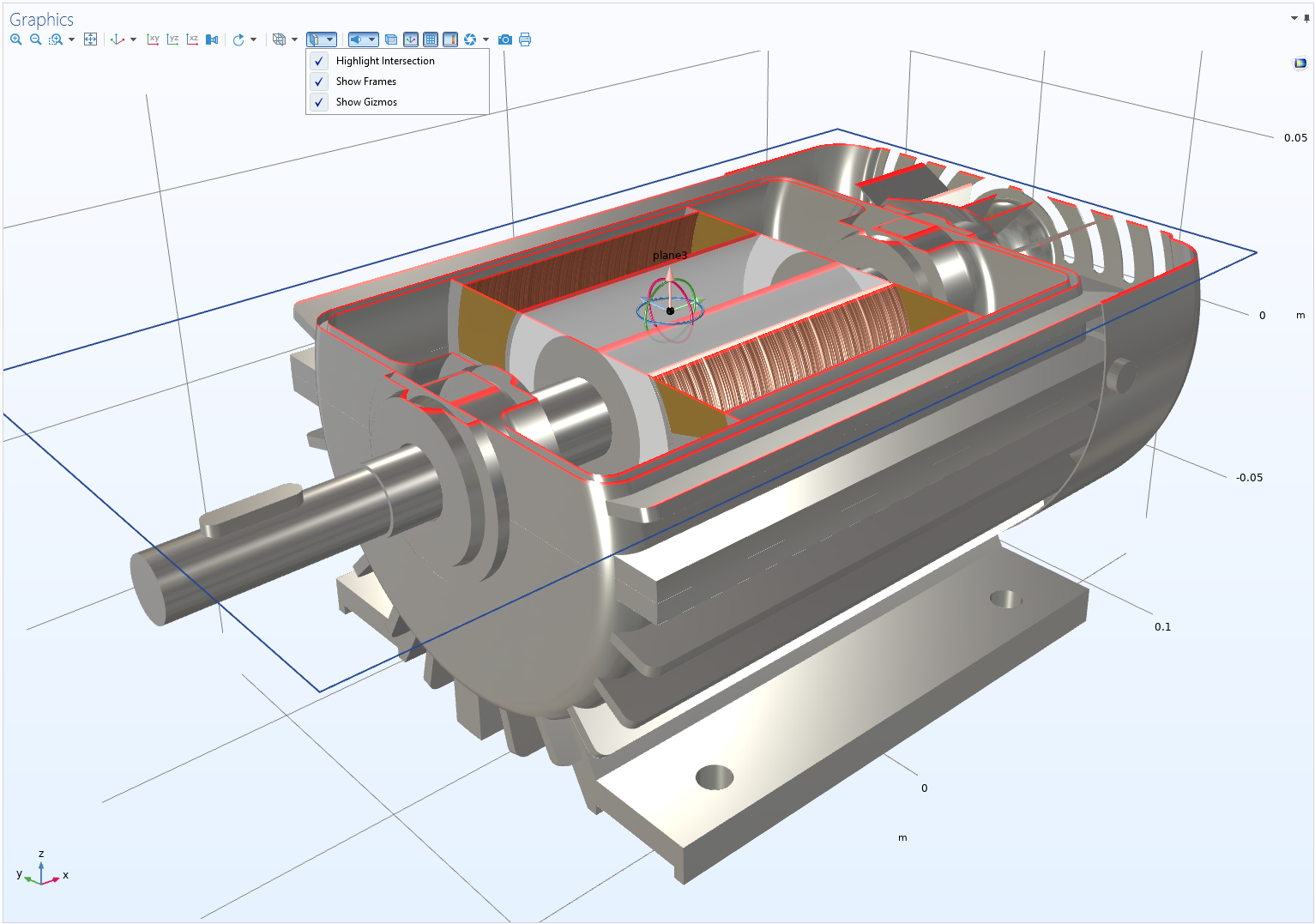
Interactive Clipping
To make it easier to select edges, boundaries, and domains that are located inside a surrounding object, you can now use interactive clipping. Add planes, boxes, cylinders, and spheres to select which parts of a geometry are shown. The interactive clipping functionality works throughout the Model Builder and is available from a menu button in the Graphics toolbar. When you click the toolbar button, by default, a Clip Plane node is added to the View node, with settings that you can adjust in a Settings window or interactively in the Graphics window. Multiple clip planes may be added and used concurrently.
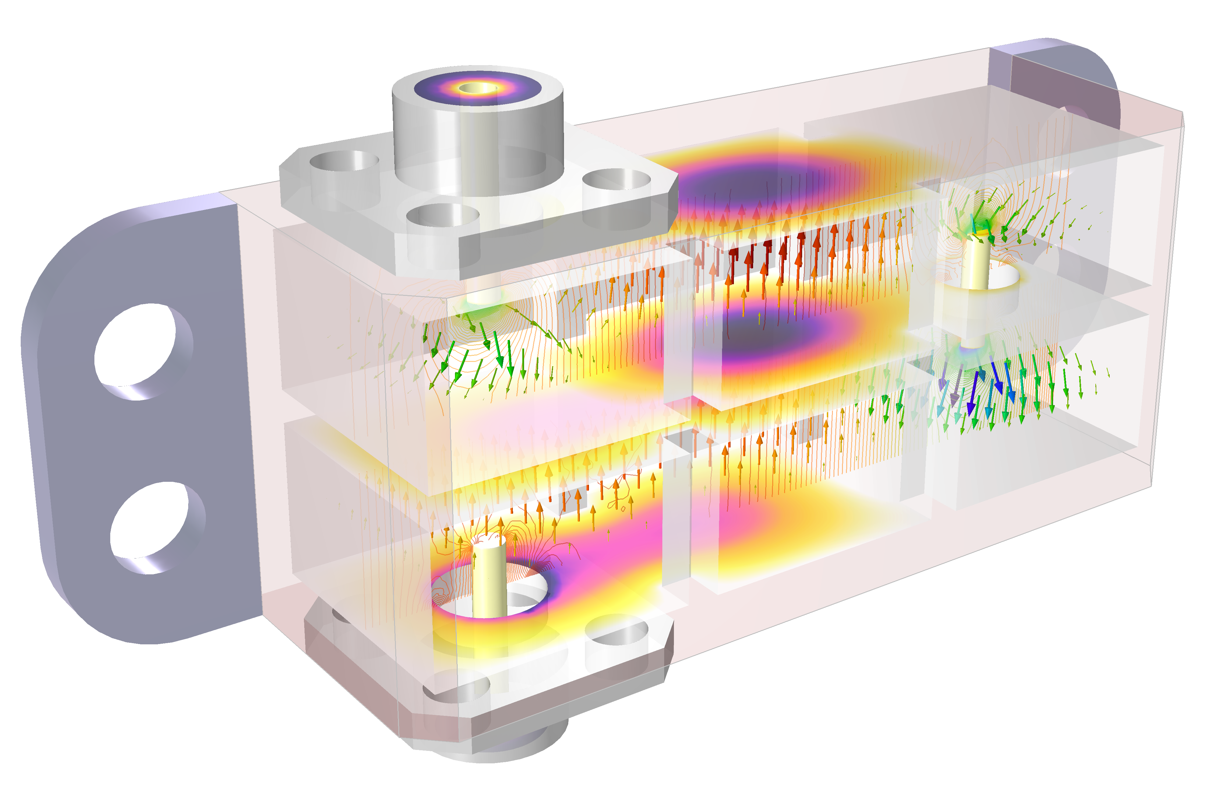
Partial Transparency
When working with 3D plots, you can now add transparency to individual plots instead of globally. By using different transparencies in each plot, you can choose which plots you want to highlight in the plot group. After adding the Transparency attribute to a plot, you can specify the amount of transparency (0–1).
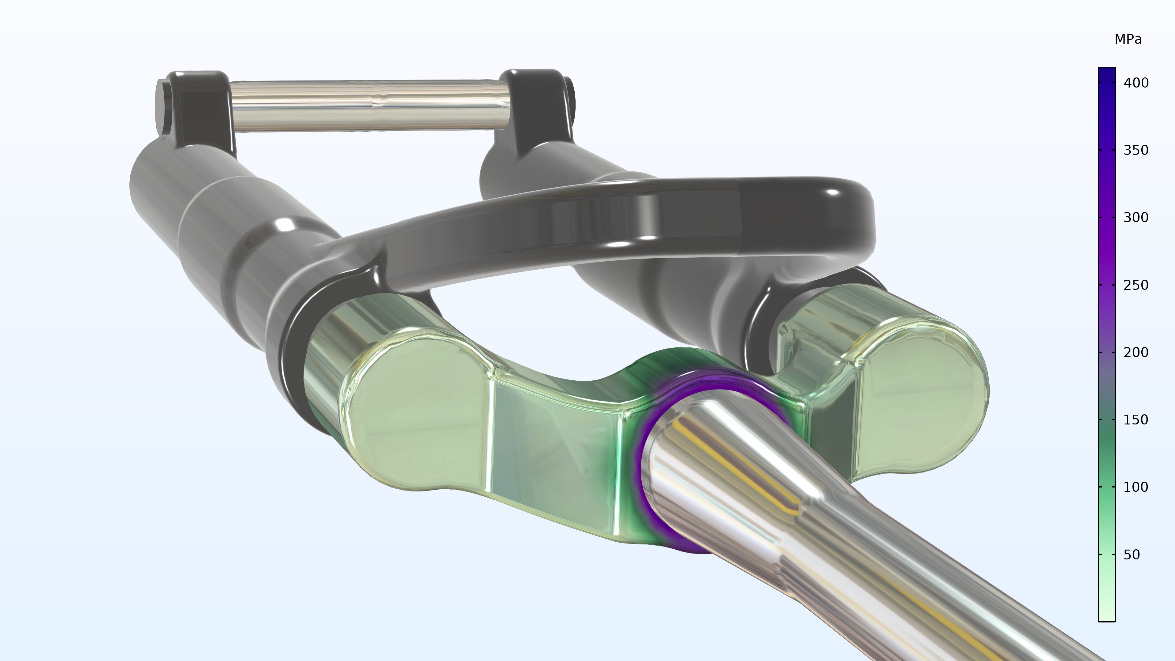
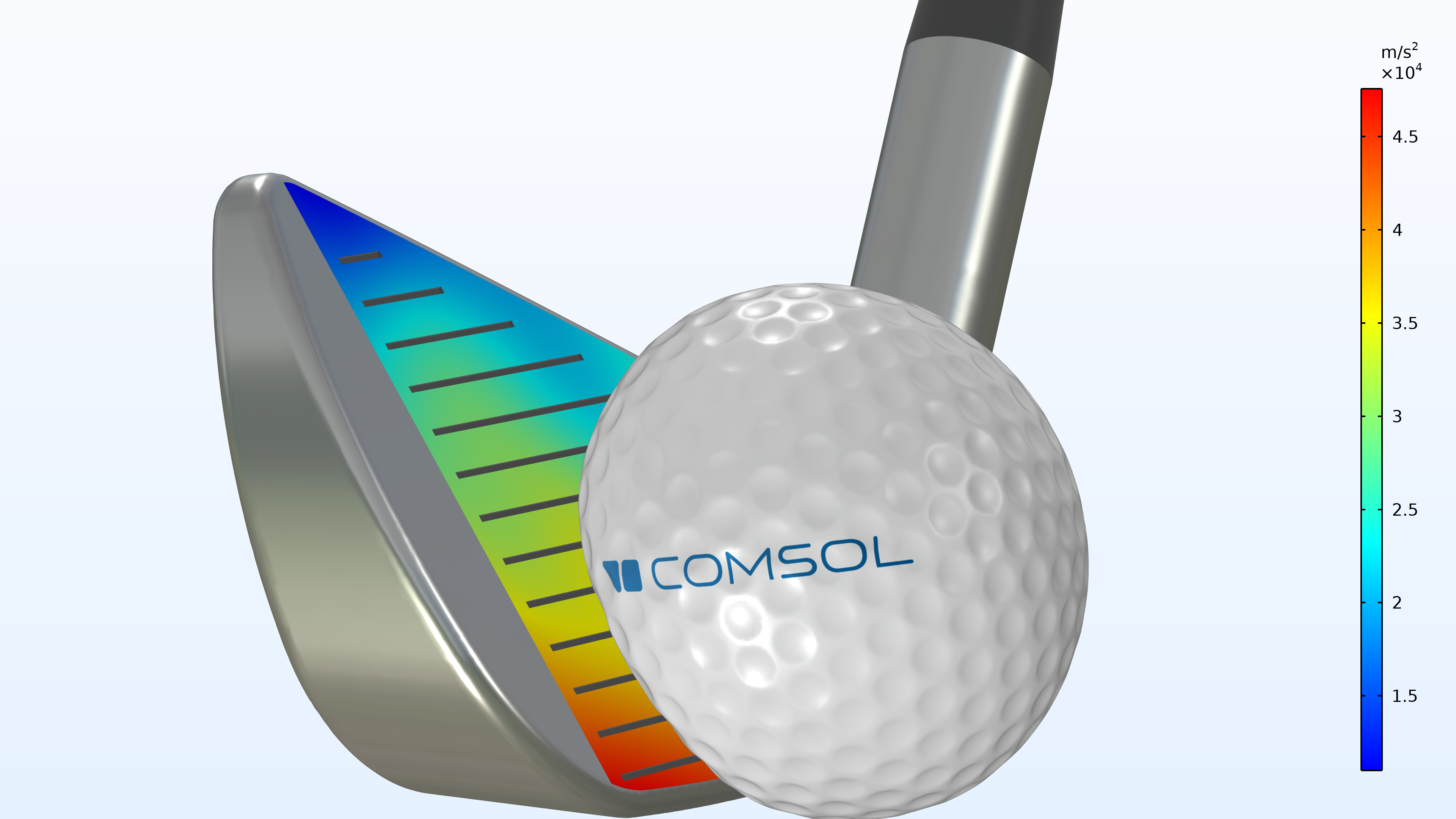
Material Appearance and Environmental Mapping in Plots
The visualization of materials is improved and support has been added for visualizing materials in plots. You are now able to create mixed visualizations where some plots show the results from a simulation while other plots show parts of the geometry using material appearance. It is also possible to mix material appearance with the plot color on a surface. The Material Appearance feature is an attribute, added to individual plots.
In addition, it is also possible to select Environment Reflections from the Graphics toolbar in order to create reflection of a predefined photorealistic environment around a device on the surface of that device. This gives a more realistic material appearance.
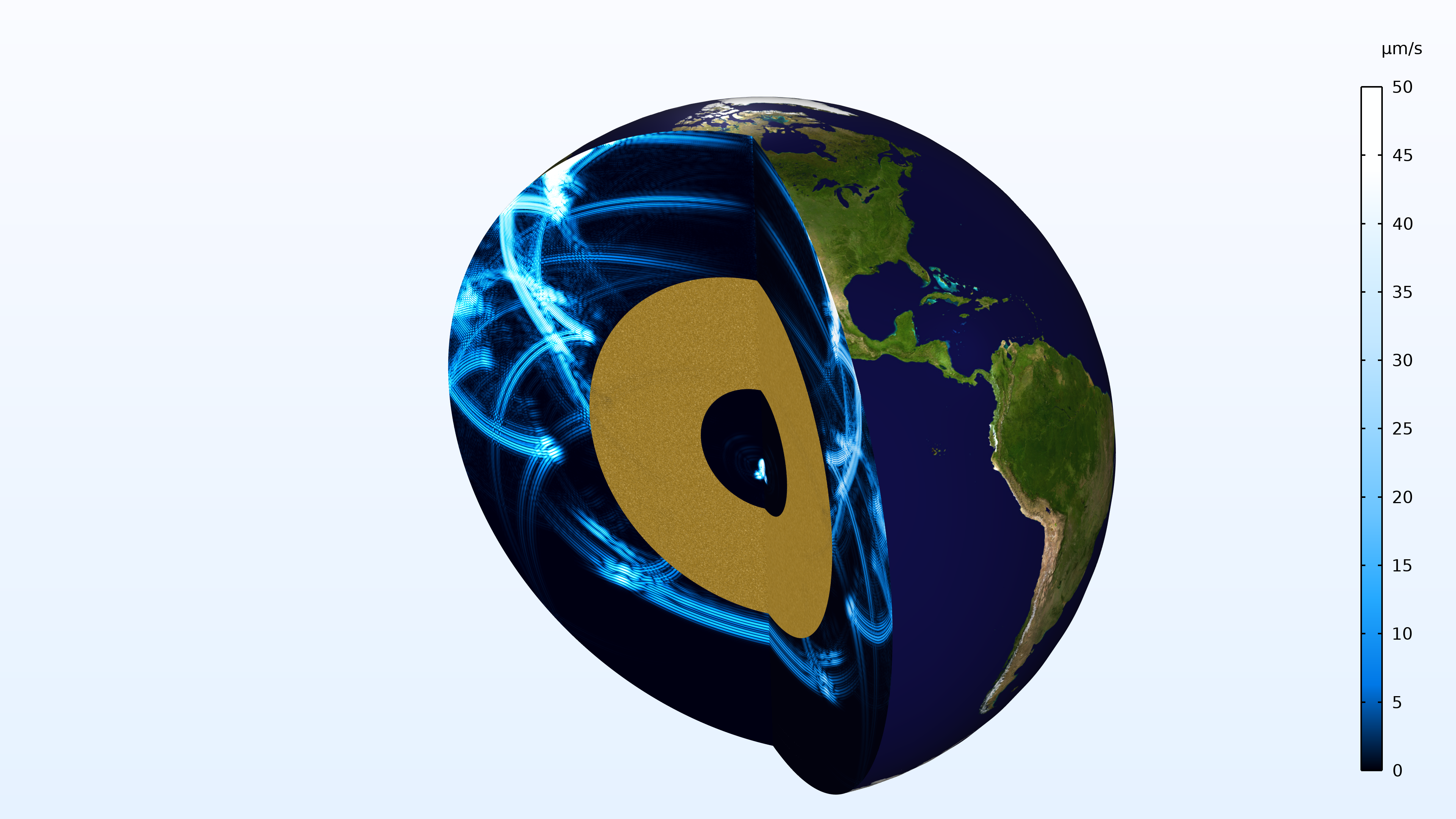
Embedding Images
You are now able to display images on surfaces in 2D and 3D. Create mixed visualizations where you combine results from a simulation with maps, background images, and more. The images can be mapped on surfaces using arbitrary expressions or predefined planar, cylindrical, and spherical mappings.
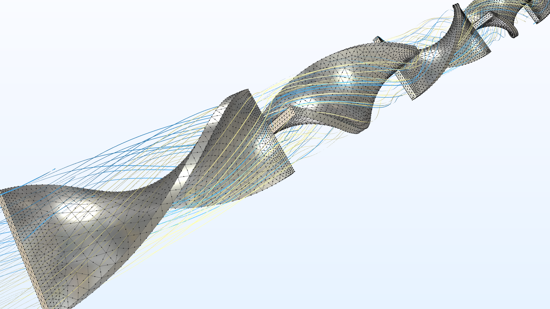
Higher-Order Elements in Mesh Plots
Mesh plots can now be used for visualizing higher-order element nodes, for fields that are solved for, as well as node points corresponding to geometry shape functions.
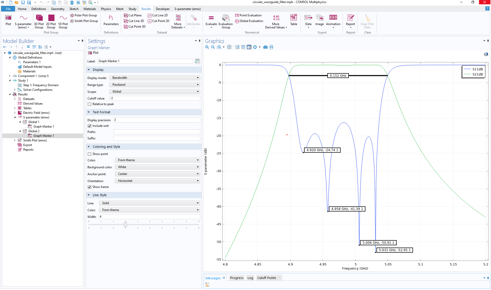
Graph Markers in 1D Plots
You can add graph markers to 1D Global and Point Graph plots that highlight both the global and local maxima and minima of a plot, and report the x-y values. You also have the option to plot the passband and stopband width in, for example, S-parameter plots. You can see this functionality demonstrated in the Detecting the Orientation of a Metallic Cylinder Embedded in a Dielectric Shell model.

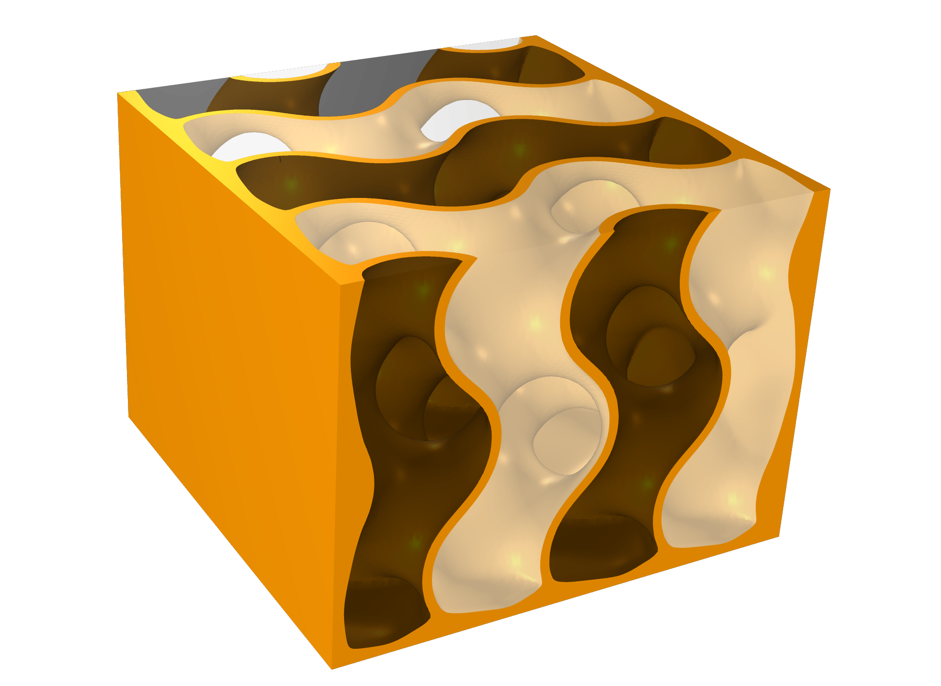
Partition Dataset
The Partition dataset is a generalization of the Filter dataset, available in previous software versions, and makes it possible to partition a domain with respect to a set of isosurfaces or contours. You can use the resulting surface mesh or volume mesh as the source for a mesh import and subsequent use in simulations. For example, you can use implicit algebraic expressions or computed field solutions to partition an object in multiple solid and fluid parts based on isolevel values. This enables multiphysics simulation on meshed geometries created using implicit modeling operations.
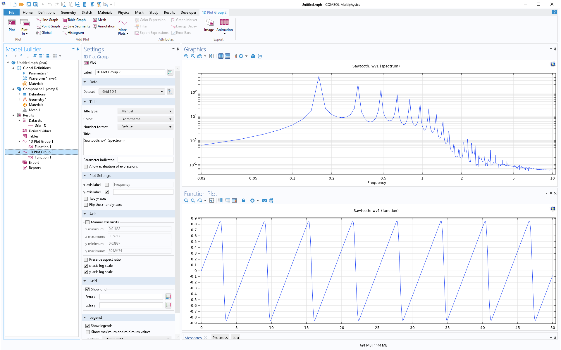
Frequency Spectrum Plot for User-Defined Functions
You can now visualize the frequency spectrum of any user-defined function, including analytic, interpolation, and waveform functions.
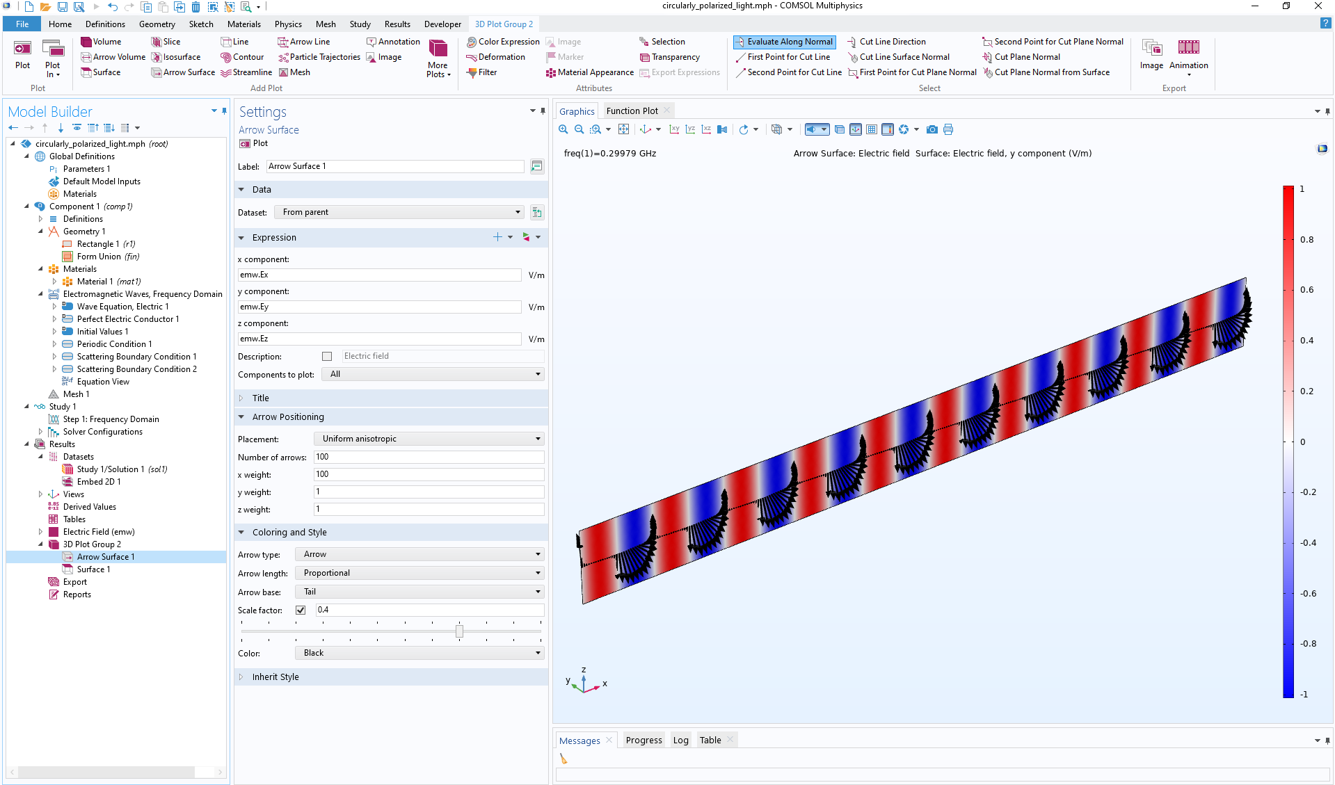
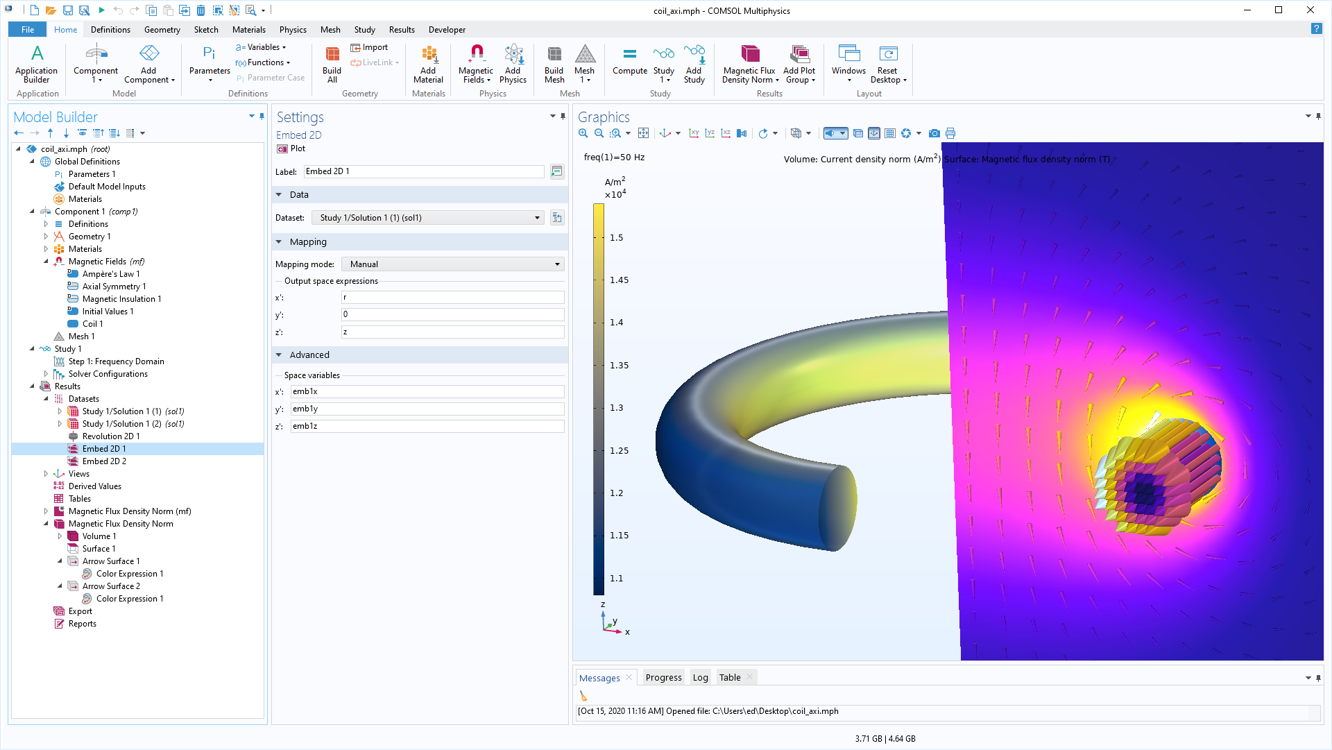
Embed Dataset
With the Embed dataset you can now embed 1D solution data into a 2D plot, and 2D solution data into a 3D plot. This is particularly useful for visualizing out-of-plane vector quantities using arrows.

Waveform Audio File Format (.wav) Export
Time-domain 1D plots can be exported to the waveform audio file format (.wav). Additionally, Impulse Response plots, available in the Acoustics Module, can be exported to this format. You can select to export as 8-bit or 16-bit, as well as change the sampling frequency.
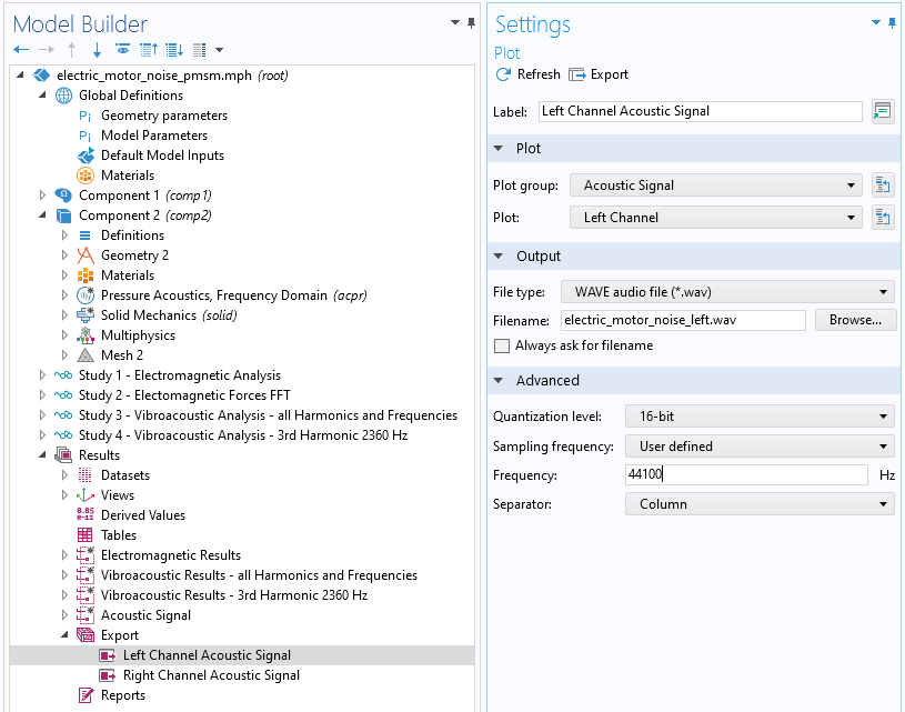
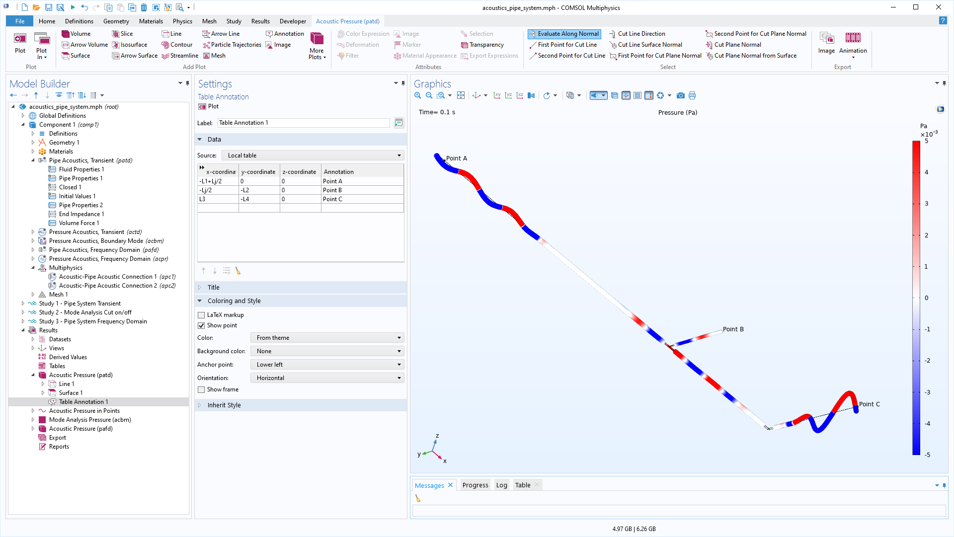
Table Annotation Plot
Display multiple annotations based on a user-defined table with the new Table Annotation plot. Coordinates for positioning the annotations can either be numbers or expressions in terms of global parameters.
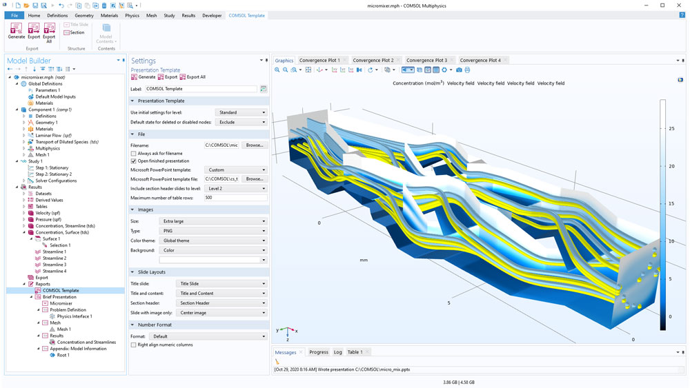
Presentations in Microsoft® PowerPoint® in Reports
The report generator can now create PowerPoint® slides that document a model and that you can use in presentations. The reports branch in the model tree allows you to define the structure of the slideshow and select the features from other parts of the model tree that you want to include. You can also add your own branded PowerPoint® template.
Additional New Functionality
- Coordinate vectors in annotations
- You can now enter coordinate vectors or use a Cut Point dataset for positioning an annotation
- Line segments in 1D plots
- By using the new Line Segments feature, you can enter a sequence of x- and y-coordinates to add auxiliary line segments to a 1D plot
- Error bars
- A new Error Bars subfeature makes it possible to add error bars to 1D global and point graph plots
- Column separators for export
- You can now control the type of column separator that is used for files created with the Export > Data and Export > Plot features
- Choose between Column, Space, Tab, Comma, Semicolon, Colon, Vertical bar (pipe)
- Point Plot
- You can visualize points as spheres, blocks, or ellipsoids at geometry vertices