CFD Module Updates
For users of the CFD Module, COMSOL Multiphysics® version 5.6 brings two new fluid flow interfaces, new options for turbulent intensity and turbulence length scale, and automatic handling of disjoint selections. Learn more about these and other new CFD features below.
Performance Improvements for Multicore and Cluster Computing
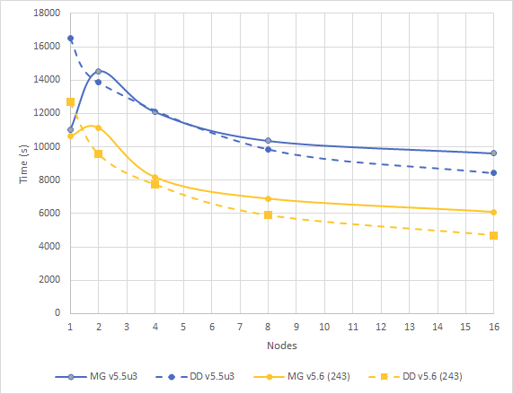
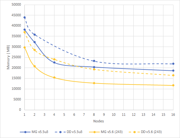
COMSOL Multiphysics® version 5.6 includes several performance improvements for the solution process. In particular, the memory requirements are reduced for Jacobian matrix assembly as well as for the algebraic multigrid preconditioner. The reduction is significant for both multicore and cluster computing. Furthermore, the most important smoothers used in the multigrid method are now more efficient, in particular for cluster computing.
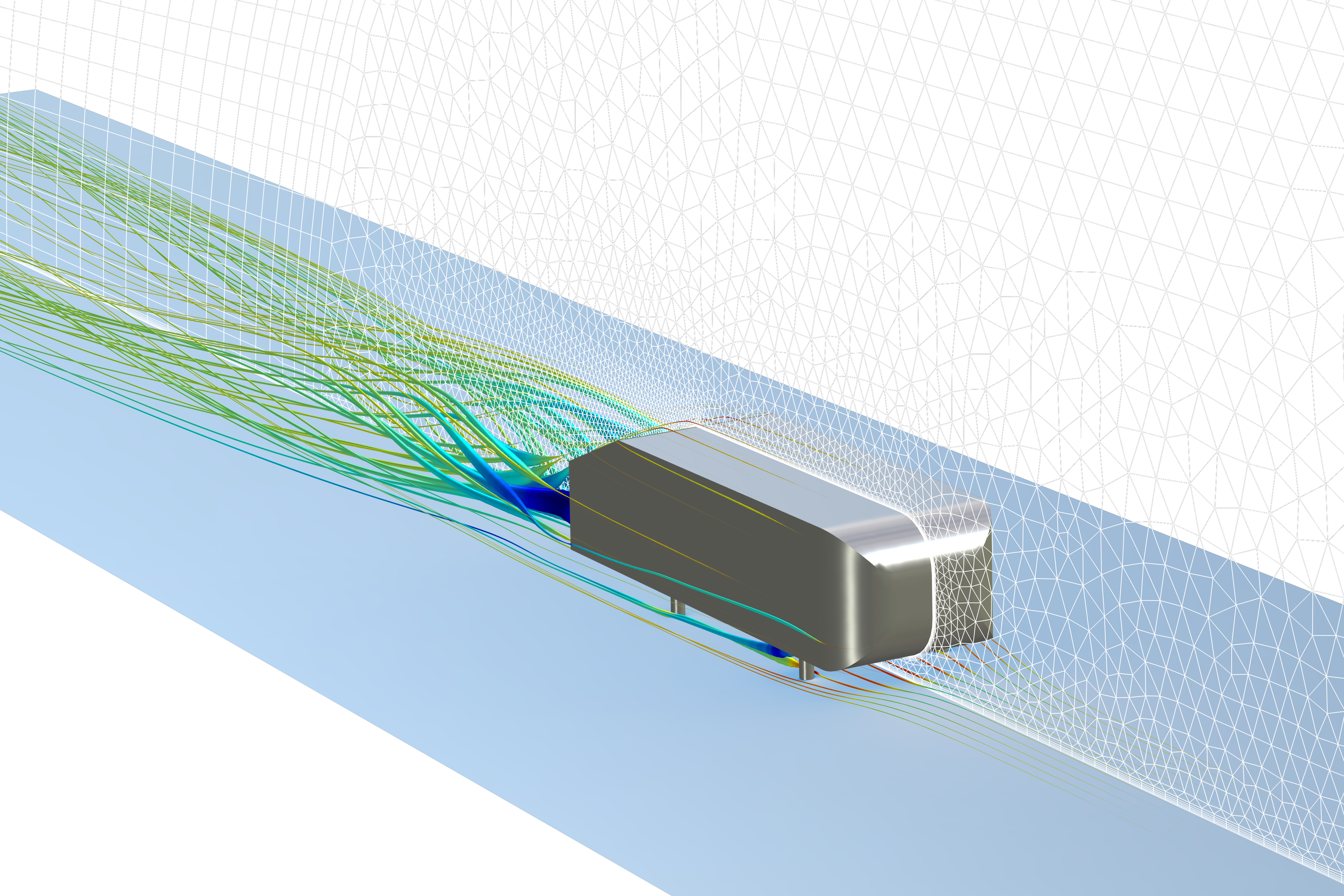
As an illustration of the improvement, consider the following CFD benchmark of an Ahmed Body featuring turbulent flow. The model used in the benchmark has a refined mesh, as compared to the Application Gallery version, with 6.3 million degrees of freedom on a 16-node cluster. In this comparison, COMSOL Multiphysics® version 5.5 update 3 and version 5.6 are installed on a cluster where each node has 48 cores (2x Intel® Xeon® Platinum 8260 24 cores). The solvers used in the comparison are the algebraic multigrid solver (SA-AMG) as a preconditioner to GMRES with the Symmetrically Coupled Gauss-Seidel smoother (denoted MG in the comparison graphs). In addition, the overlapping Domain Decomposition (Schwarz) method is used as a preconditioner to GMRES with the multigrid method as a domain solver (denoted DD). The graphs below show the performance as computation time vs. number of nodes and memory usage vs. number of nodes.
Compressible Dispersed Multiphase Flow
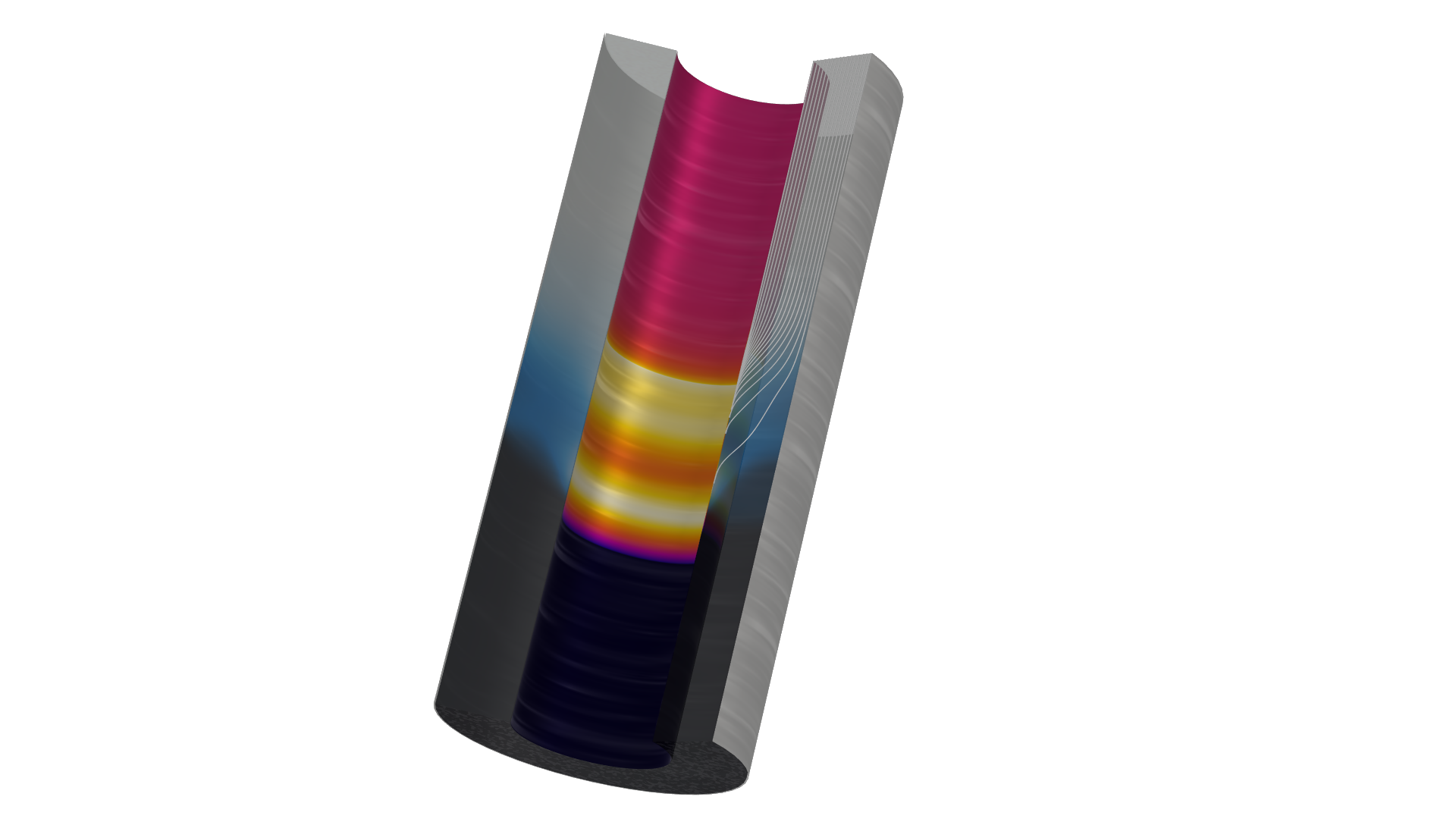
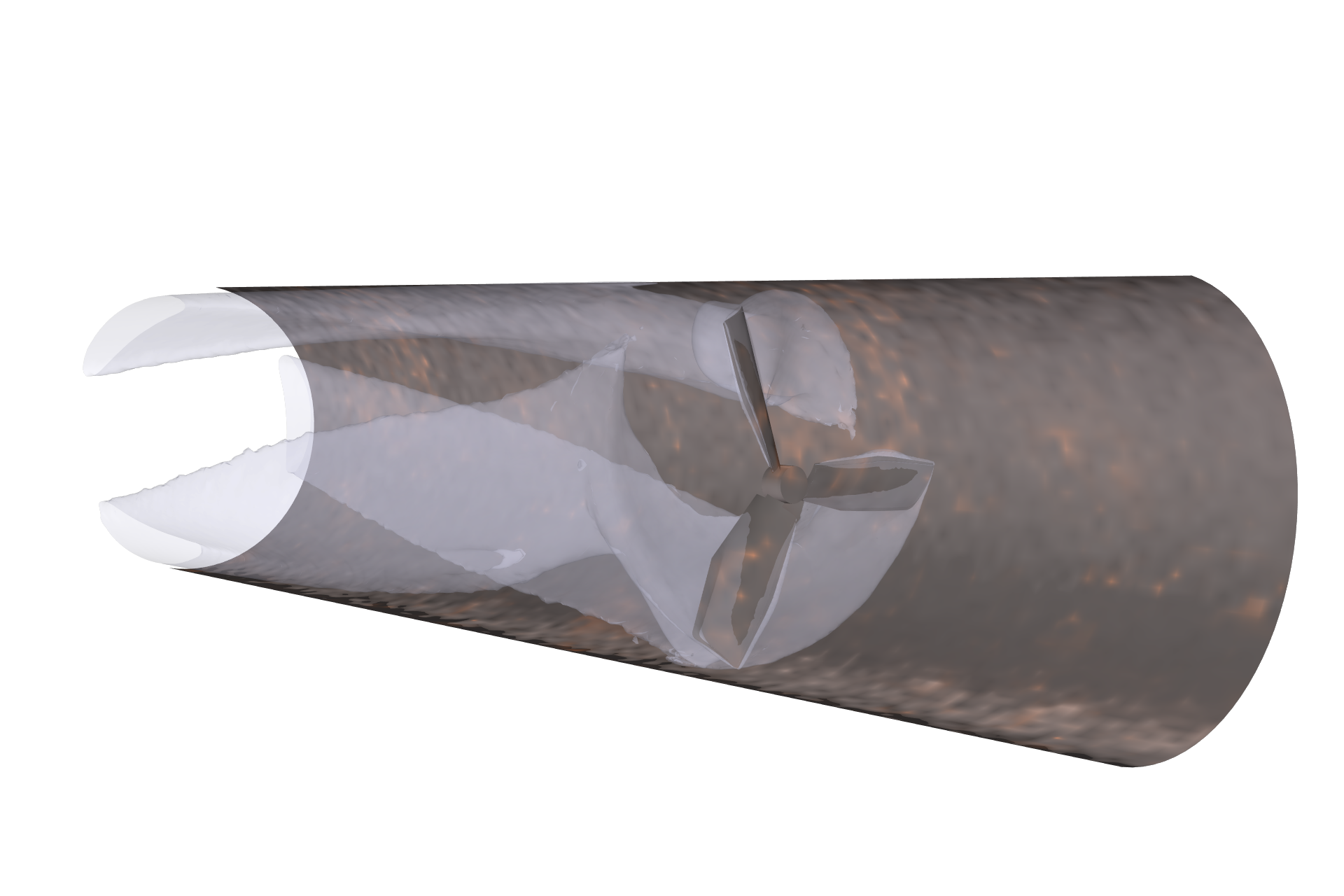
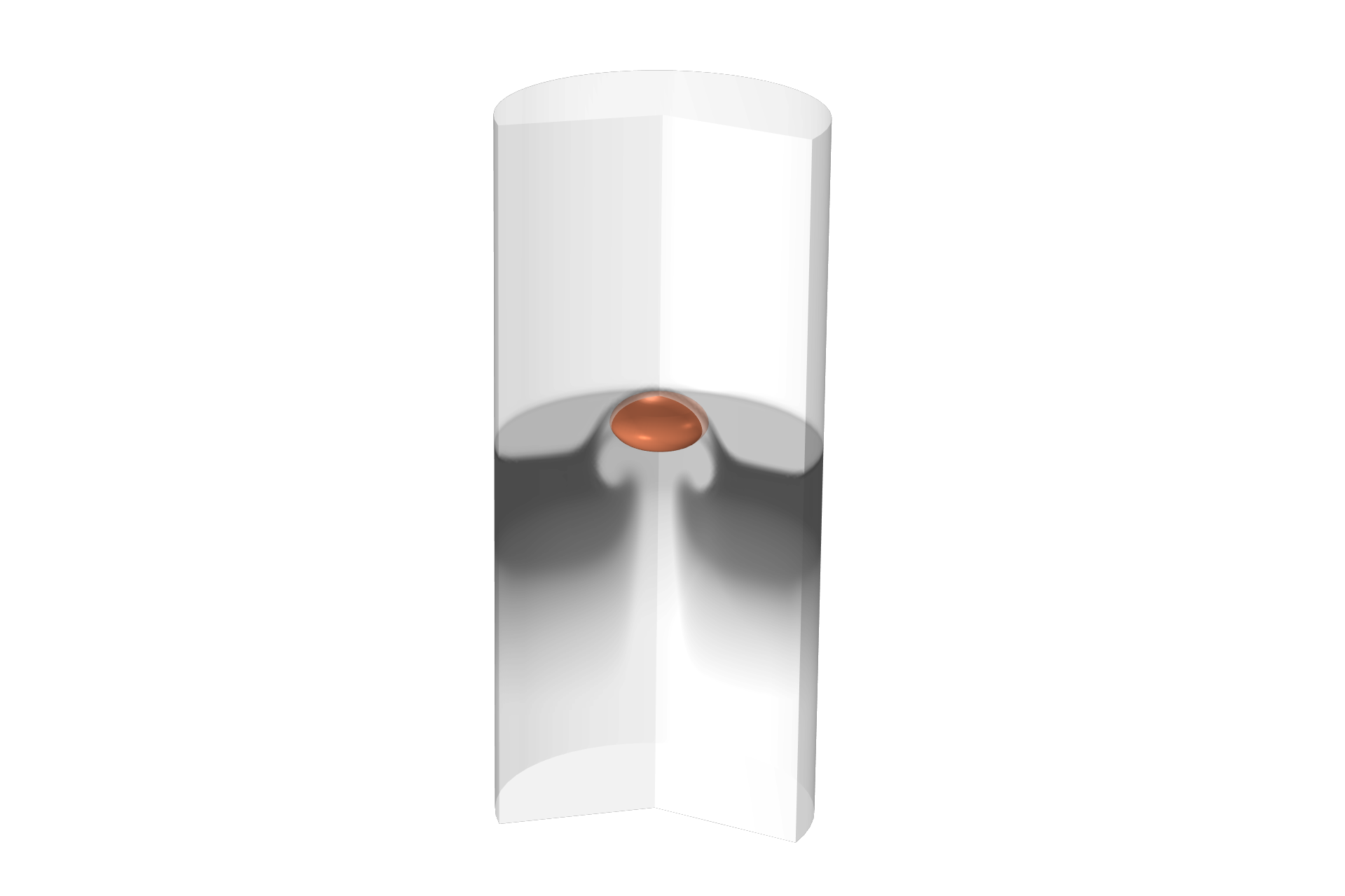
Many natural phenomena, manufacturing processes, and separation processes involve dispersed multiphase flows with particles, bubbles, or droplets transported by a continuous phase. The Phase Transport, Mixture Model interfaces, which allow for an arbitrary number of dispersed phases, have been revised to support compressible mixture flows. These flow interfaces also have improved support for deforming and rotating domains. Additionally, the Phase Transport, Mixture Model interface can now be used together with the level set method in simulations that combine a separated and dispersed modeling approach. You can view this updated formulation feature in the new Droplet Rising Through a Suspension tutorial model.
An oil droplet rising through a suspension. The suspension is initially stratified, with a dense layer between two clear layers, and the droplet is initially located in the bottom clear layer. This model demonstrates the combination of a dispersed multiphase flow model with a level set model.
Nonisothermal Mixture Model
Simulating processes in which bubbles are formed in a liquid, such as nucleate boiling or cavitation processes, requires the coupling of multiphase flow with heat transfer. The new Nonisothermal Mixture Model interfaces provide exactly this functionality: They couple a Laminar Flow or Turbulent Flow (RANS) interface, a Phase Transport interface, and a Heat Transfer in Fluids interface using the new Nonisothermal Flow, Mixture Model and Nonisothermal Mixture Model multiphysics coupling nodes. All RANS turbulence models are supported by the Nonisothermal Mixture Model interfaces.
Shallow Water Equations
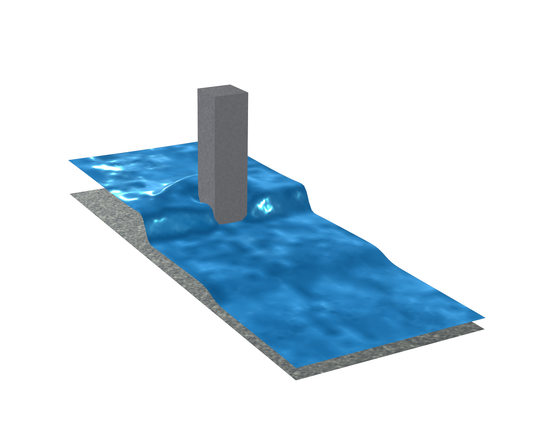
The shallow water approximation is frequently applied in oceanographic and atmospheric applications to predict effects of tsunami impacts, areas affected by pollution, coastal erosion, and polar ice-cap melting, to mention a few. The new Shallow Water Equations, Time Explicit interface uses a depth-averaged formulation to solve free-surface flows in 1D and 2D domains. The bottom topography in a model can conveniently be defined from a digital elevation model (DEM). You can see this feature in the new Tsunami Runup onto a Complex 3D Beach, Monai Valley tutorial model.
Tsunami impact simulated with the Shallow Water Equations, Time Explicit interface.
Total Pressure Condition
For certain applications, such as in pump simulations, it is more convenient to specify the total (or stagnation) pressure on inlet and outlet boundaries. COMSOL Multiphysics® version 5.6 includes options for imposing either pointwise values or average values of the total pressure on inlets and outlets for incompressible flow.
New Averaging Options for Fluid Properties Across Phase Interfaces
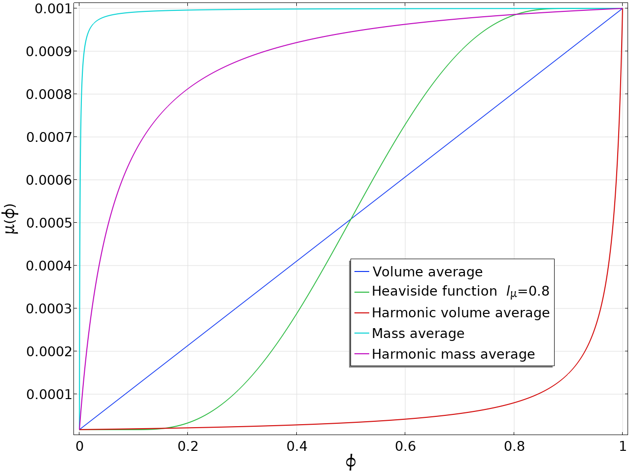
When the density and/or viscosity ratio in a two-phase flow simulation is large, the use of volume-averaged fluid properties across the phase interface may lead to excessive smearing. Sharpening the transition zone for the fluid properties, or displacing it into one of the two phases, may improve accuracy and/or convergence in some cases. In version 5.6, smoothed Heaviside functions and harmonic volume averages can be used for both density and viscosity. For the viscosity, mass averaging and harmonic mass averaging are also available as options.
New Options for Turbulence Conditions
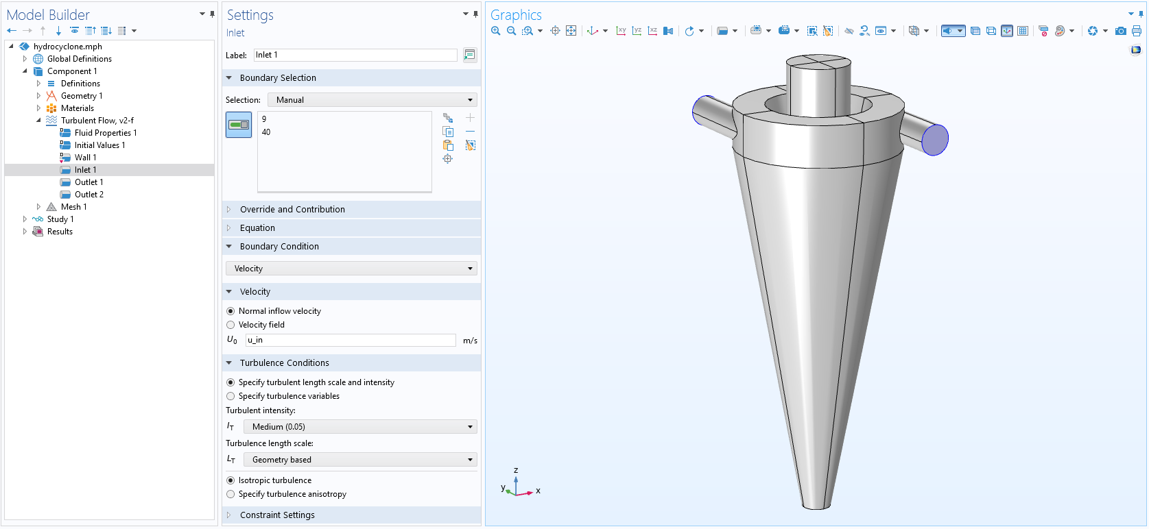
Three new options are available for the turbulent intensity on inlets and open boundaries: Low (0.01), Medium (0.05), and High (0.1). There is also a new Geometry based default option for the turbulence length scale on inlets. This option automatically calculates the hydraulic diameter of the inlet and sets the turbulence length scale to 0.07 times the hydraulic diameter, which is the recommended value for fully developed turbulent flow in pipes and channels.
Automatic Handling of Disjoint Selections
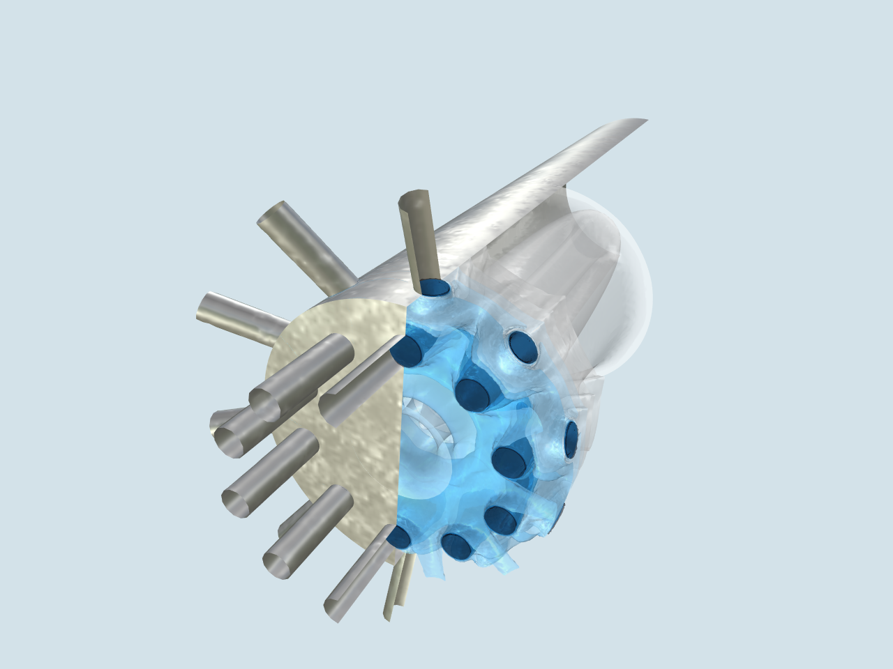
For Fully Developed Flow on inlets and outlets, and Mass Flow on inlets, a selection consisting of disjoint boundaries can be handled within a single boundary feature. This new default option adds one equation for each connected component in a selection. The connected components in a disjoint selection are detected automatically.
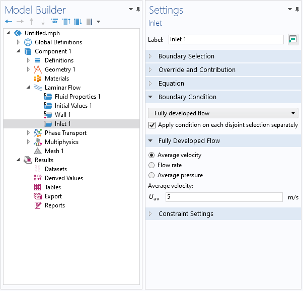
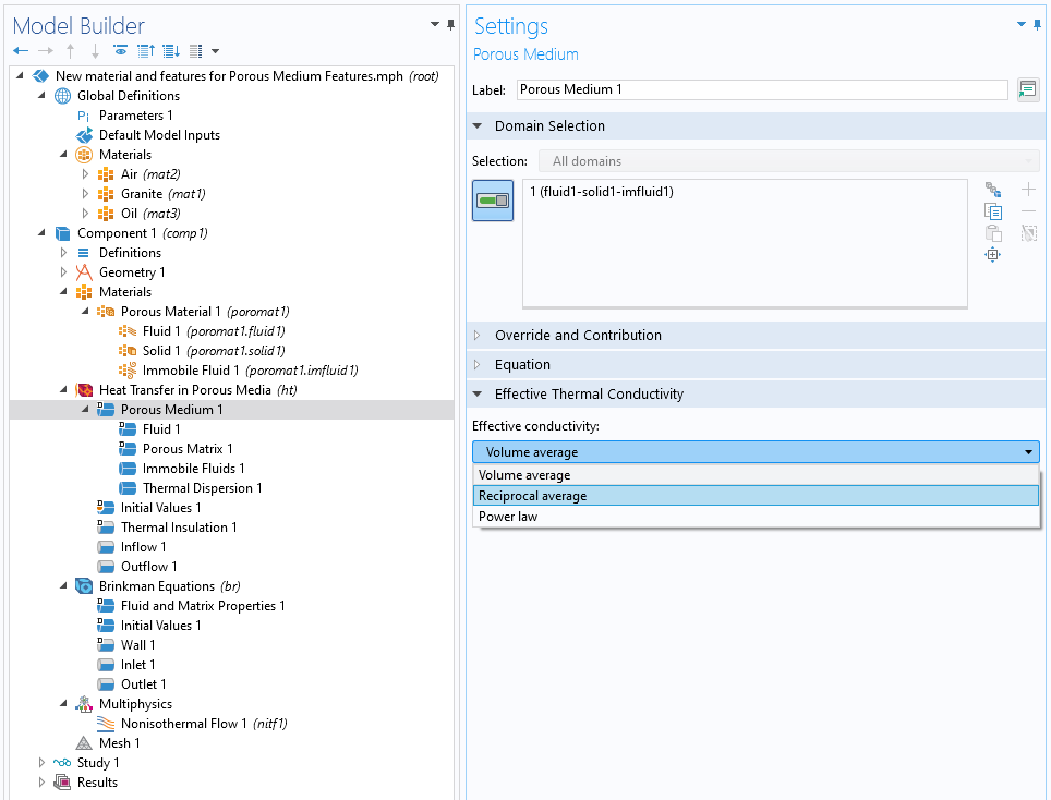
New Porous Medium Feature
A new feature for handling a porous medium is available for defining the different phases: solids, fluids, and immobile fluids. In the Heat Transfer in Porous Media interface, the Porous Medium feature is used to manage the material structure with a dedicated subfeature for each phase: Fluid, Porous Matrix, and optionally, Immobile Fluids. This new workflow provides added clarity and improves the user experience. It also facilitates multiphysics couplings in porous media in a more natural way. Combined with the Moisture Transport and Porous Media Flow interfaces, the heat transfer in porous media improvements enable the modeling of nonisothermal flow and latent heat storage in porous media.
You can see this new setup in the following models:
- heat_pipe
- frozen_inclusion
- evaporation_porous_media_large_rate
- porous_microchannel_heat_sink
- convection_porous_medium
- carbon_deposition
- monolith_3d
- steam_reformer
Automatic Detection of Ideal Gas Material in Heat Transfer in Fluids
The Fluid feature, available within the various heat transfer interfaces, has been updated to take advantage of the ideal gas assumption to improve computational efficiency. The new From material option of the Fluid type list automatically detects whether the material applied on each domain selection is an ideal gas or not, and uses the relevant properties for either case. This may speed up computation when computing pressure work in compressible nonisothermal flows, for example. Since the gases available in COMSOL Multiphysics® and in the Material Library are modeled as ideal gases, many models with compressible nonisothermal flow are expected to benefit from this improvement.
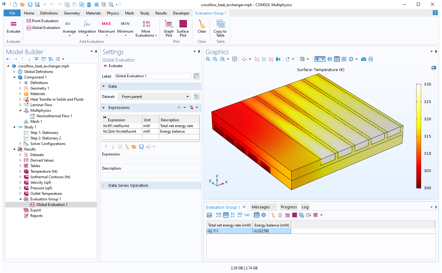
Heat and Energy Balance
The postprocessing variables for energy and heat balance definition have been extended to cover new configurations. Specifically, the variables are for nonisothermal flow, to account for out-of-plane heat sources; for the work of volume forces, viscous dissipation, and pressure; for boundary stresses; and for enthalpy flux in cases of nonzero normal velocity on internal walls. The postprocessing variables or energy and heat balance definition have also been extended to layered materials. Energy and heat balance provide an alternative criterion to the solver error estimate to check the simulation accuracy. You can see this functionality demonstrated in the Electronic Chip Cooling model.
Easier Setup for Phase Field and Level Set Models
The Level Set and Phase Field interfaces have been restructured: Two Initial Values nodes are now added by default, and the previously used Initial Interface feature has been removed. Instead, the initial interface is automatically placed at the boundaries between the two Initial Values nodes with different initial phases.

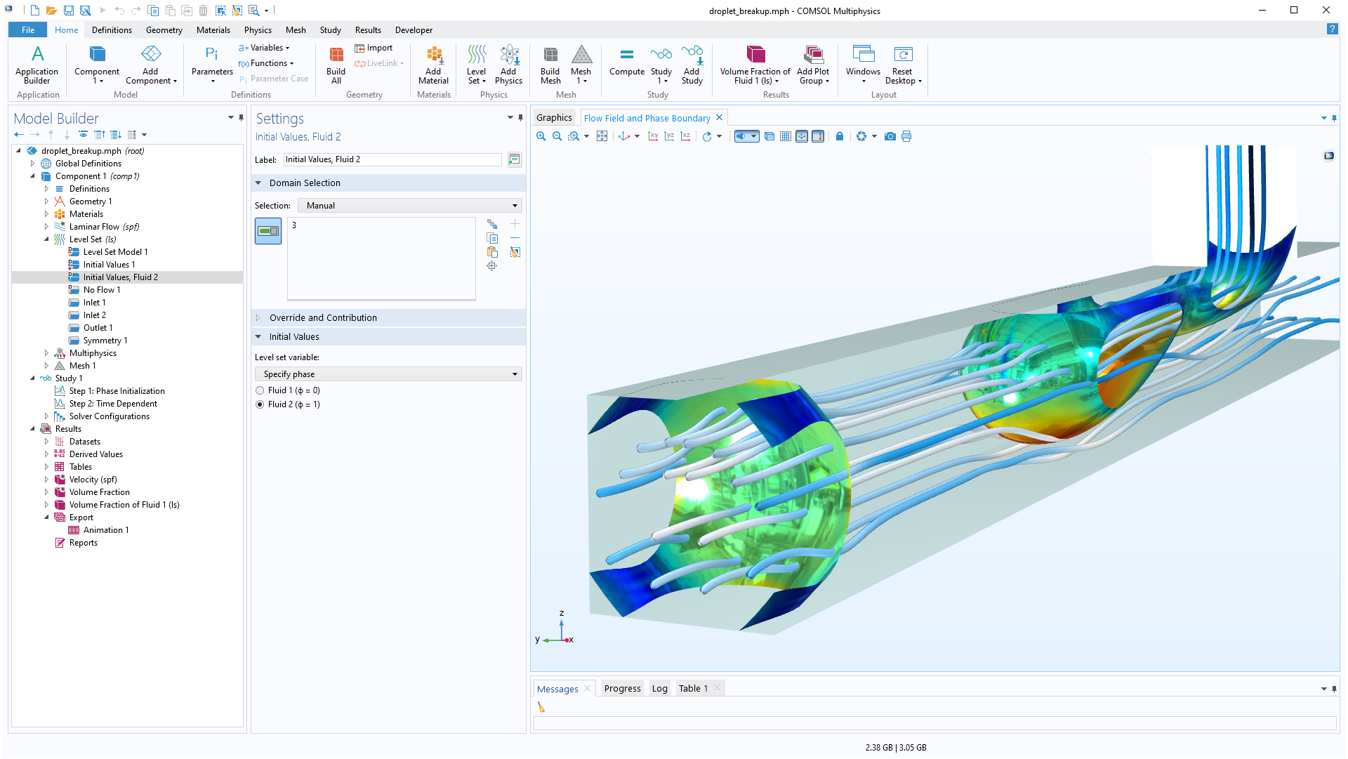
Settings for the Initial Values, Fluid 2 feature. Note that the Initial Interface feature is no longer needed. The initial distribution of the level set or phase field function is solved for in the Phase Initialization study step.
New Tutorial Models
COMSOL Multiphysics® version 5.6 brings several new tutorial models to the CFD Module.
Droplet Rising Through a Suspension
Application Library Title:
droplet_rising_through_a_suspension
Download from the Application Gallery
Polymer Electrolyte Membrane Electrolyzer
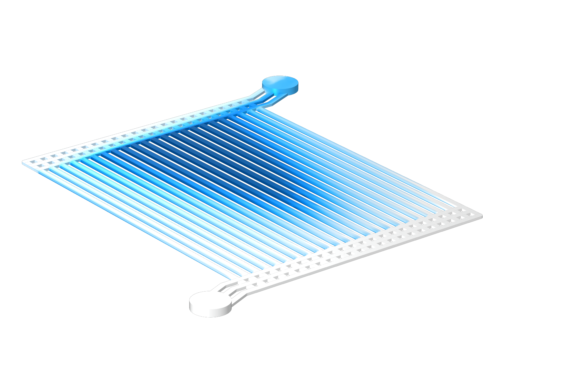
polymer_electrolyte_membrane_electrolyzer
Download from the Application Gallery
Dam Breaking on a Column, Shallow Water Equations
Application Library Title:
dam_break_column_sw
Download from the Application Gallery
Tsunami Runup onto a Complex 3D Beach, Monai Valley

Application Library Title:
monai_runup
Download from the Application Gallery