Acoustics Module Updates
For users of the Acoustics Module, COMSOL Multiphysics® version 5.6 brings a new Nonlinear Acoustics, Time Explicit interface, a Port boundary condition for elastic wave propagation, and nonlinear effects in transient thermoviscous simulations. Learn about these and more acoustics updates below.
Nonlinear Acoustics, Time Explicit for High Sound Pressure Levels
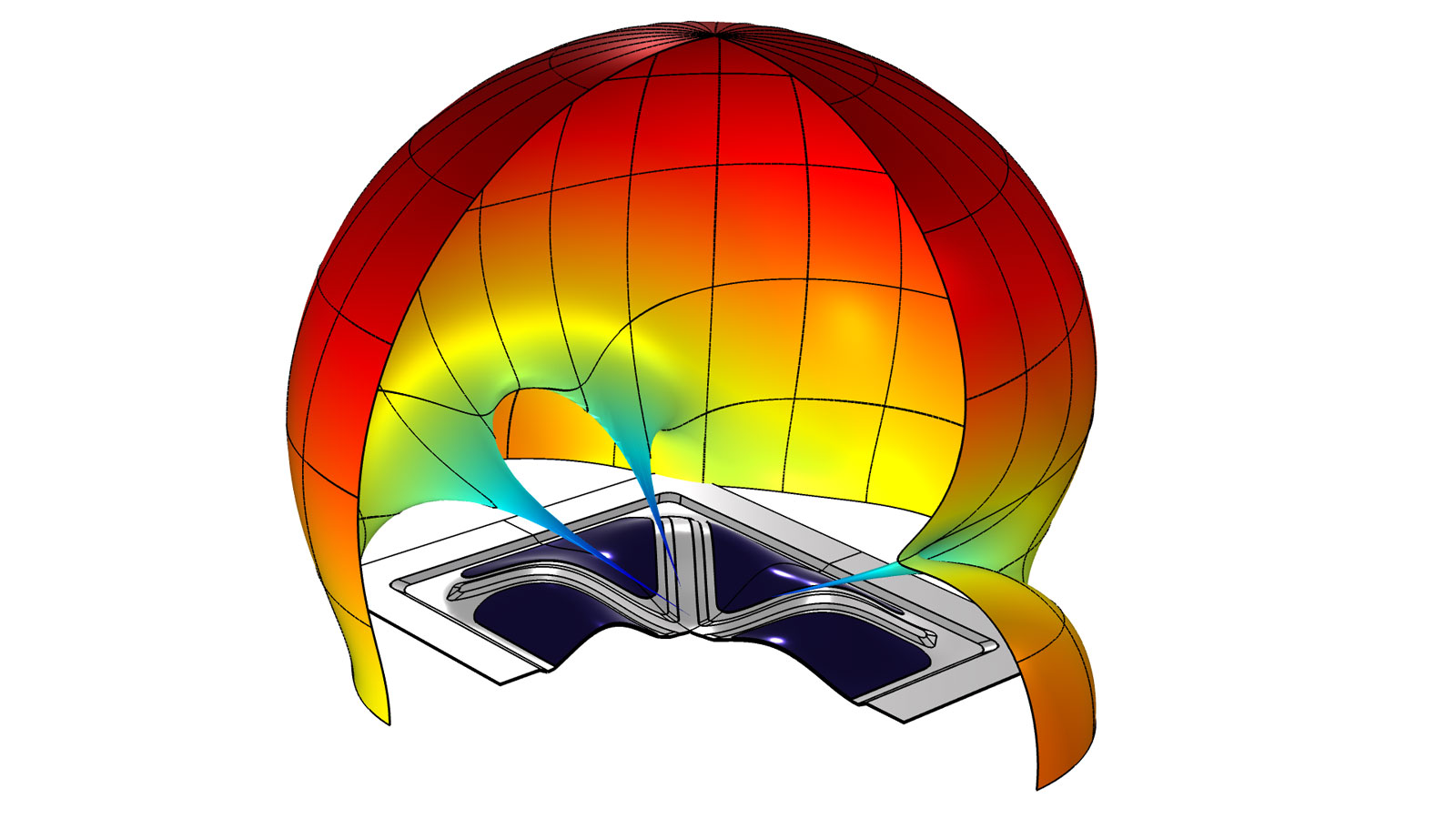
The new Nonlinear Acoustics, Time Explicit interface is used for modeling finite-amplitude high sound-pressure-level nonlinear waves in fluids. Application areas include biomedical areas, for instance, ultrasonic imaging and high-intensity focused ultrasound (HIFU), but also any acoustic system with nonlinear effects due to a high level of excitation. The method is very memory efficient and can solve problems with many million degrees of freedom (DOFs).
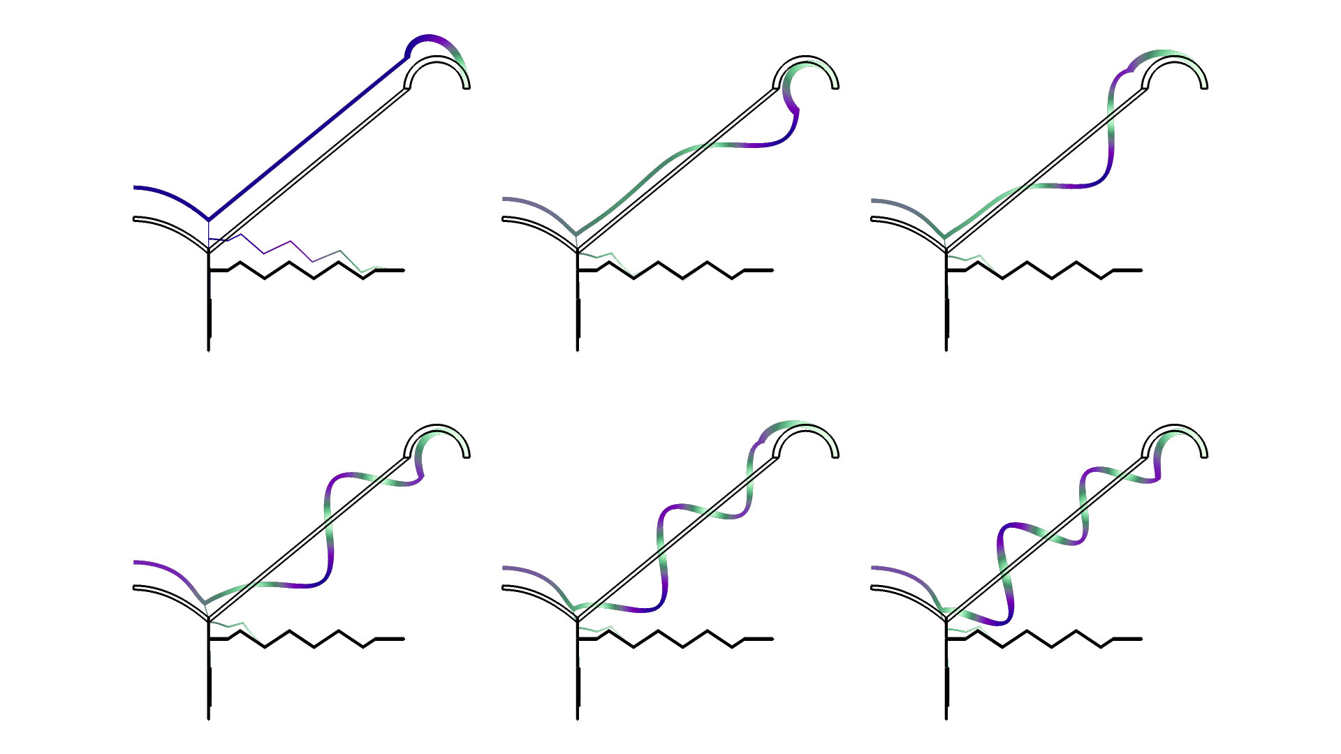
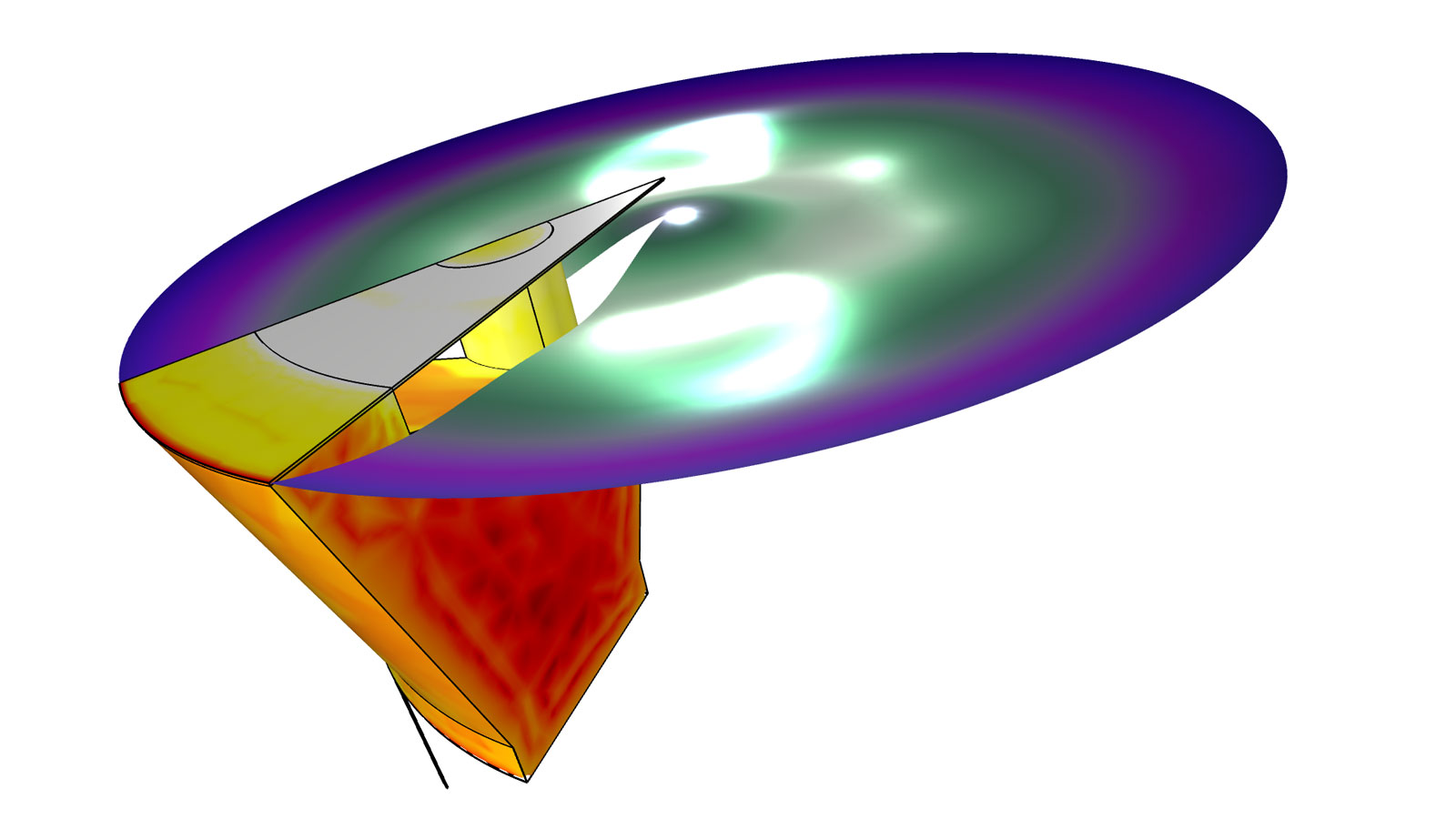
The interface is multiphysics enabled and can be coupled with the Elastic Waves, Time Explicit interface to model vibroacoustic problems. Absorbing layers are used to set up effective nonreflecting boundary conditions. Consistent handling of material discontinuities is enabled when modeling transitions between materials such as different tissues and fluids, for example. You can see this interface in the new Nonlinear Propagation of a Cylindrical Wave — Verification Model and High-Intensity Focused Ultrasound (HIFU) Propagation Through a Tissue Phantom tutorial models.
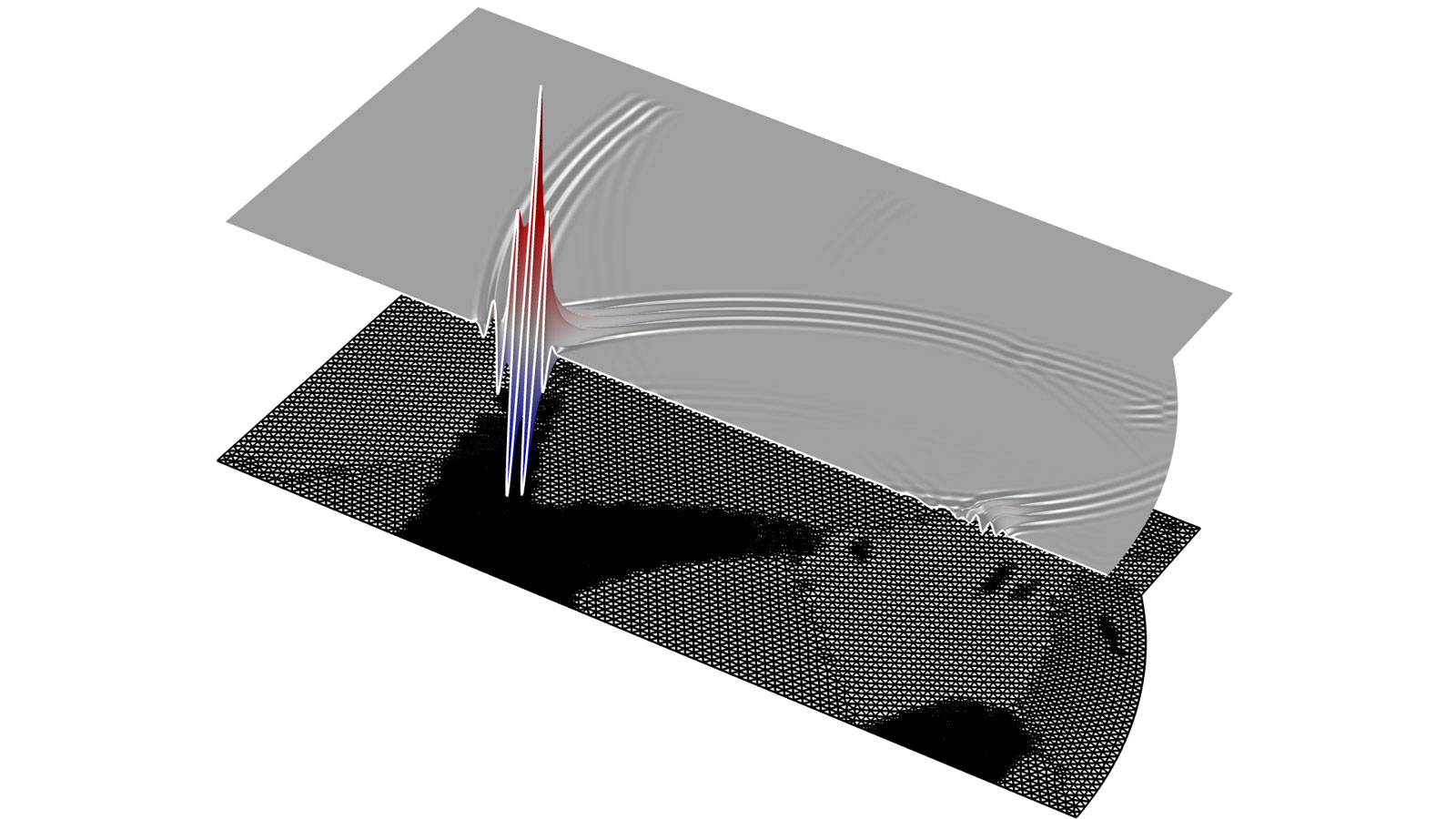
Animation of the propagation of a focused ultrasonic pulse in a tissue sample. The mesh is depicted and shows how the adaptive mesh refinement ensures correct resolution of the focused signal (the dark regions have a very fine mesh). The mesh is only updated when necessary.
Port Boundary Condition for Elastic Wave Propagation
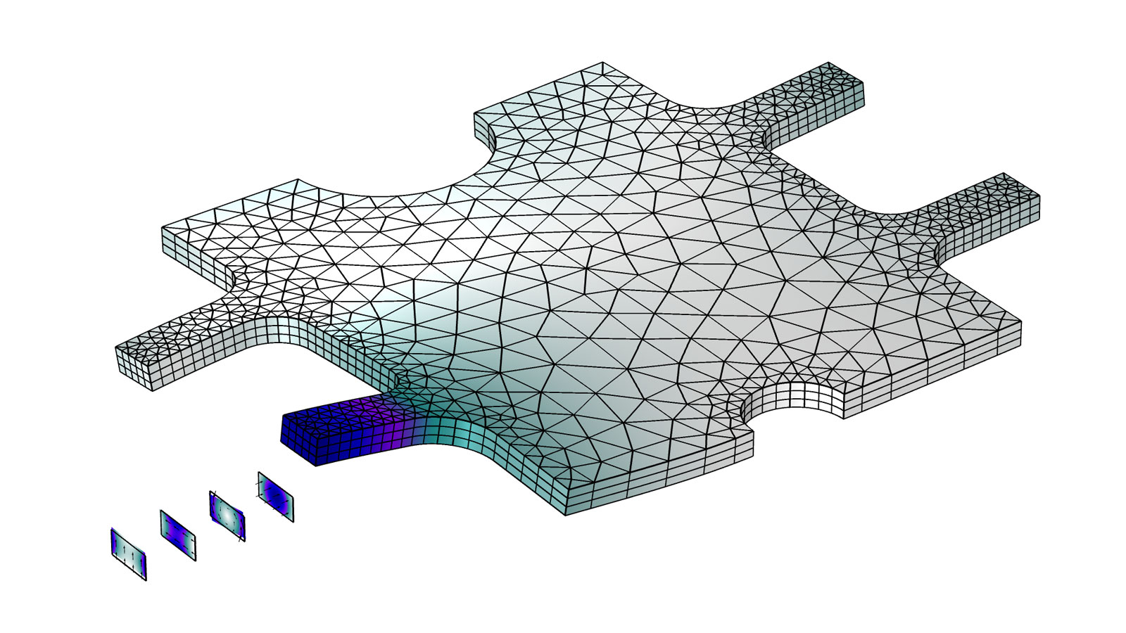
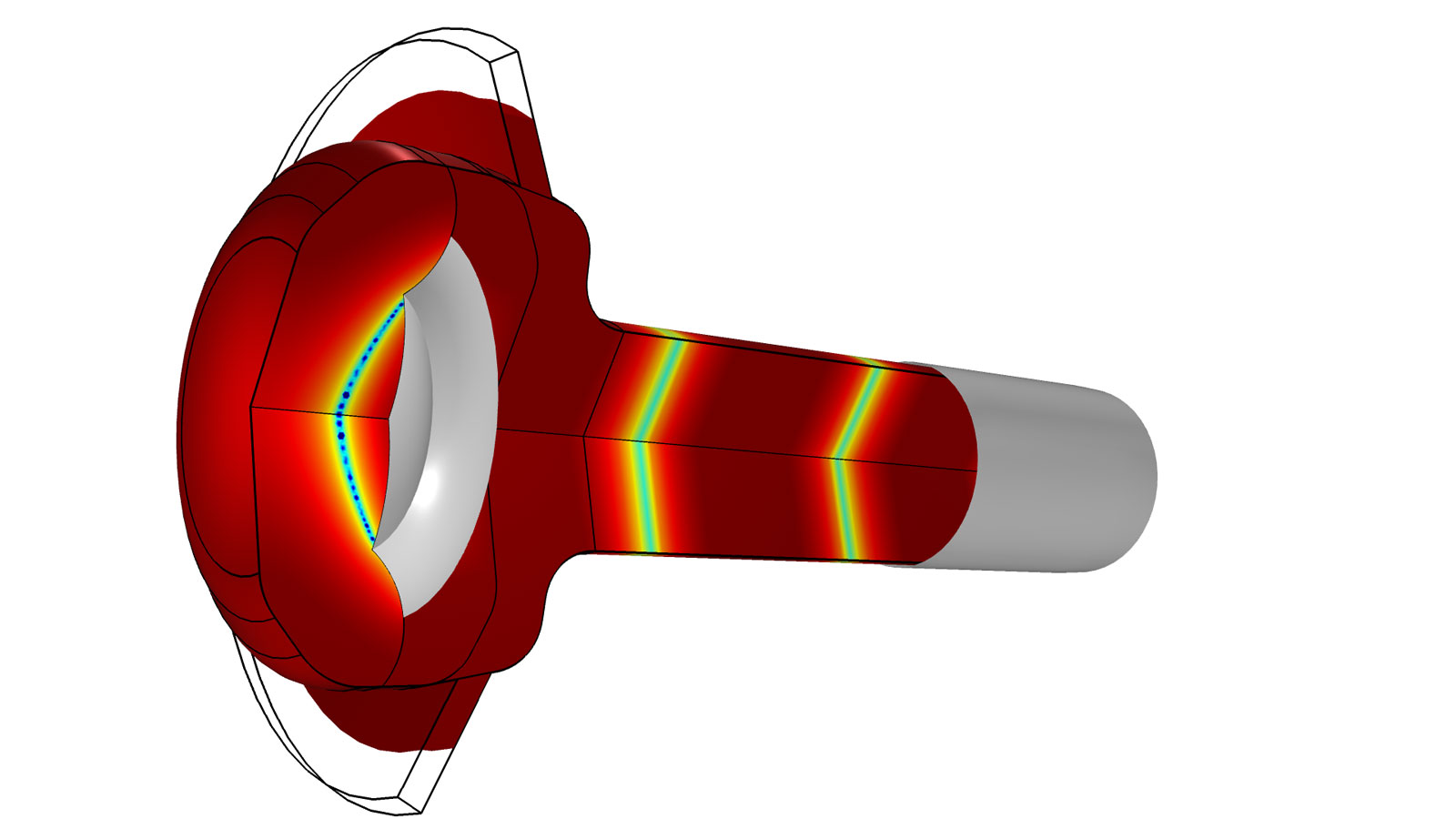
The new Port boundary condition, available with the Solid Mechanics interface, is designed to excite and absorb elastic waves that enter or leave solid waveguide structures. A given Port condition supports one specific propagating mode. Combining several Port conditions on the same boundary allows a consistent treatment of a mixture of propagating waves, for example, longitudinal, torsional, and transverse modes. The combined setup with several Port conditions provides a superior nonreflecting condition for waveguides to a perfectly matched layer (PML) configuration or the Low-Reflecting Boundary feature, for example. The port condition supports S-parameter (scattering parameter) calculation, but it can also be used as a source to just excite a system. The power of reflected and transmitted waves is available in postprocessing. To compute and identify the propagating modes, the Boundary Mode Analysis study is available in combination with the port conditions. You can view this functionality in the new Mechanical Multiport System: Elastic Wave Propagation in a Small Aluminum Plate tutorial model.

Nonlinear Thermoviscous Acoustics for Miniature Sound Ports, Perforates, and Grills
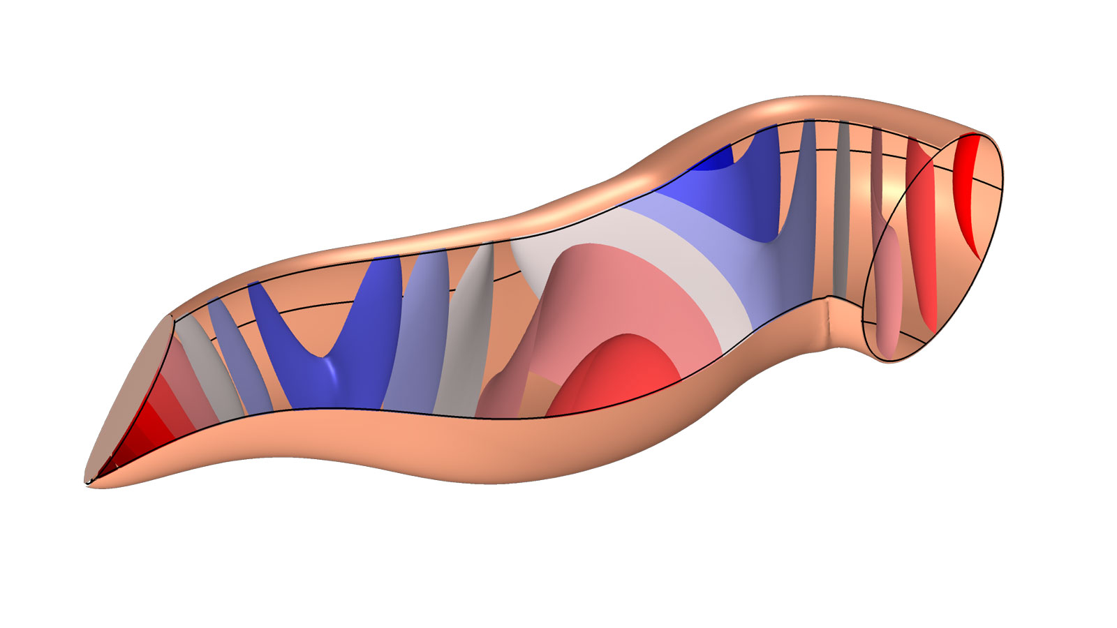
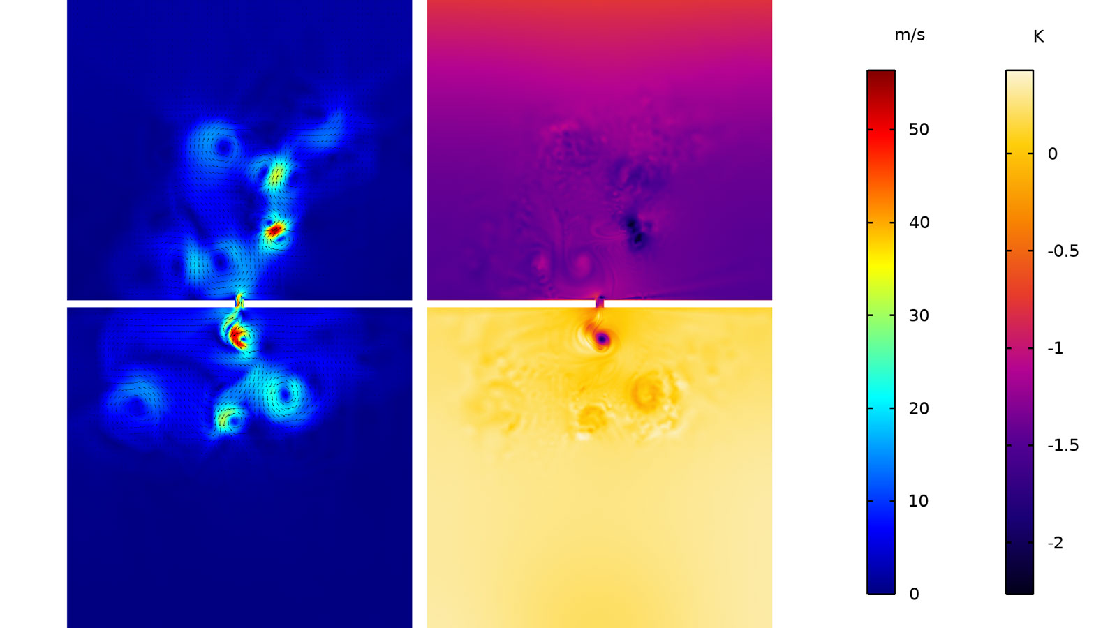
The Nonlinear Thermoviscous Acoustics Contributions feature adds the necessary contributions to the Thermoviscous Acoustics, Transient interface in order to model nonlinear effects in a transient thermoviscous simulation. The contributions allow for the modeling of vortex shedding that may happen at sudden expansions, like in a perforate, a grill, or at a miniature sound port. Vortex shedding or separation, generated by the acoustic field, generally introduces distortion in the measured response of a system by creating higher-order harmonics. With the second-order density representation option, the feature can also capture the nonlinear effect associated with high sound pressure levels that require a nonlinear representation of the equation of state (the pressure, density, and temperature relation). Stabilization has been added to the thermoviscous acoustics interfaces, which is essential when using the Nonlinear Thermoviscous Acoustics Contributions feature for solving highly nonlinear problems. You can see this new feature in the updated Nonlinear Slit Resonator tutorial model.
Acoustic velocity (left) and temperature (right) perturbations showing vortex shedding as a large amplitude pressure wave interacts with a small narrow slit.
Lumped Port Boundary Condition in Pressure Acoustics
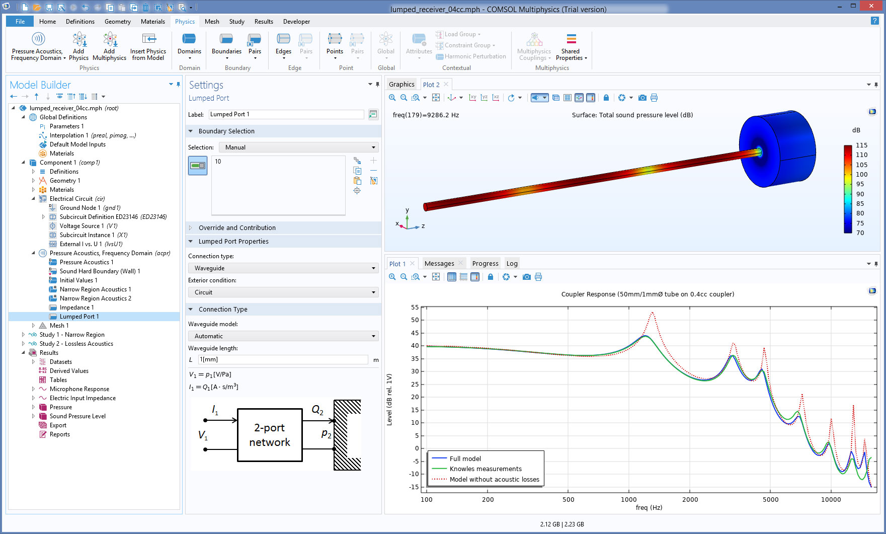
The new Lumped Port boundary condition in the Pressure Acoustics, Frequency Domain interface connects the end of a waveguide or duct inlet/outlet to an exterior system with a lumped representation. This can be an Electrical Circuit (with the AC/DC Module), a two-port network defined through a transfer matrix, or a lumped representation of a waveguide. Several representations and sources exist to describe the lumped system and to excite the system. When using the lumped port representation, it is assumed that only plane waves propagate in the acoustic waveguide. The condition simplifies, for example, setting up electroacoustic models where transducers or subsystems are described through a lumped equivalent model. This can be when modeling the miniature loudspeakers integrated into earbuds or hearing aids, or when modeling microphones and their inlet in smart speaker systems. You can see this new feature in these two updated models:
- lumped_receiver_with_full_vibroacoustic_coupling
- lumped_receiver_connected_to_test_setup_with_a_0.4_-_cc_coupler
More Powerful Boundary Element Method (BEM) for Large Acoustics Models
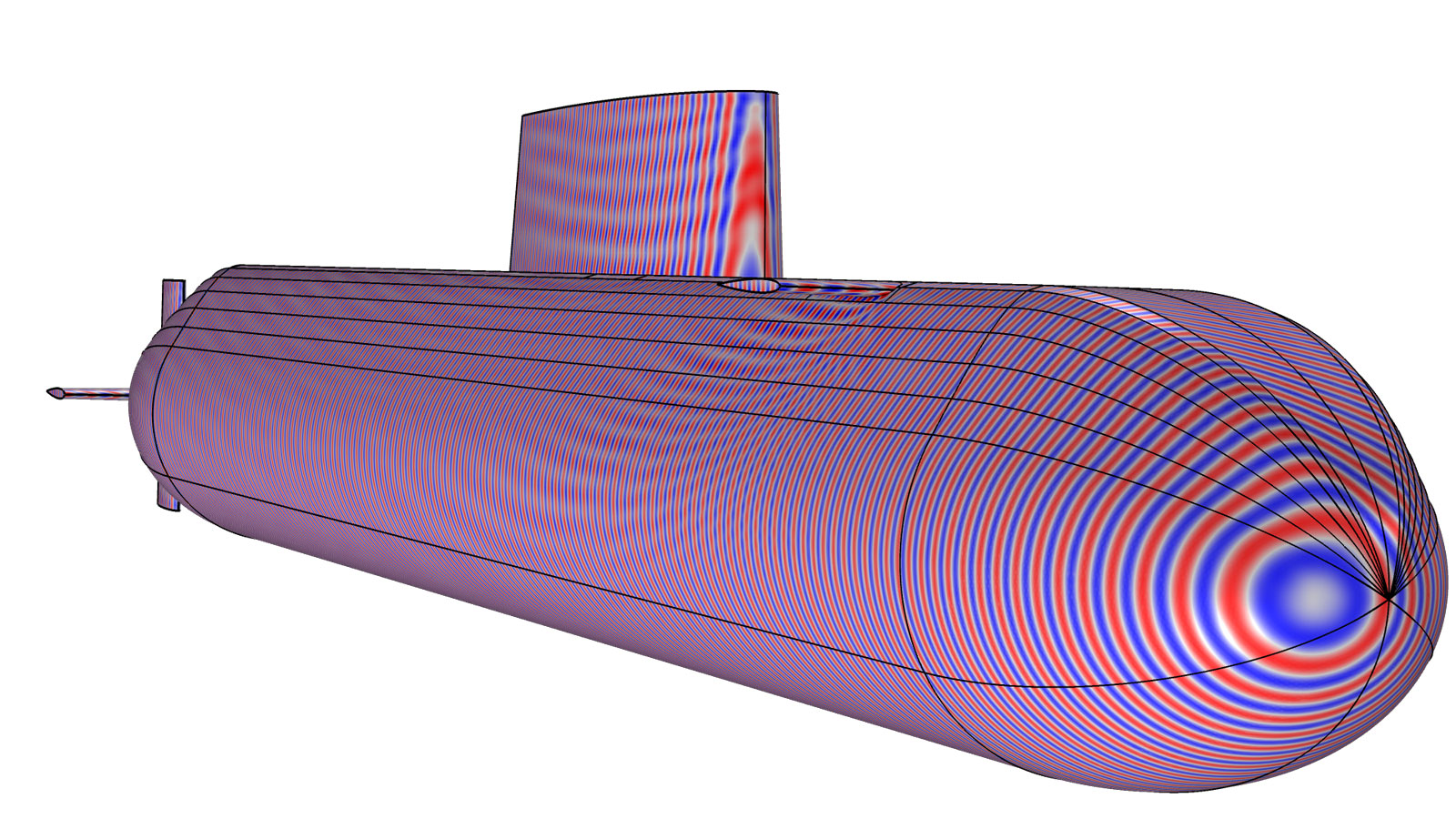
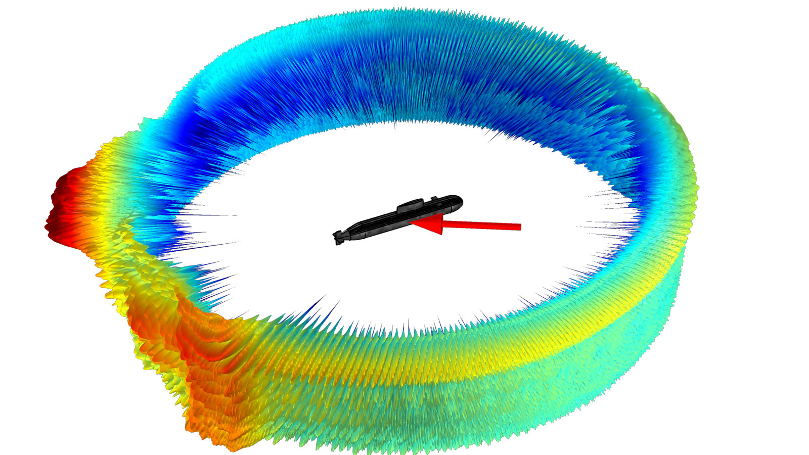
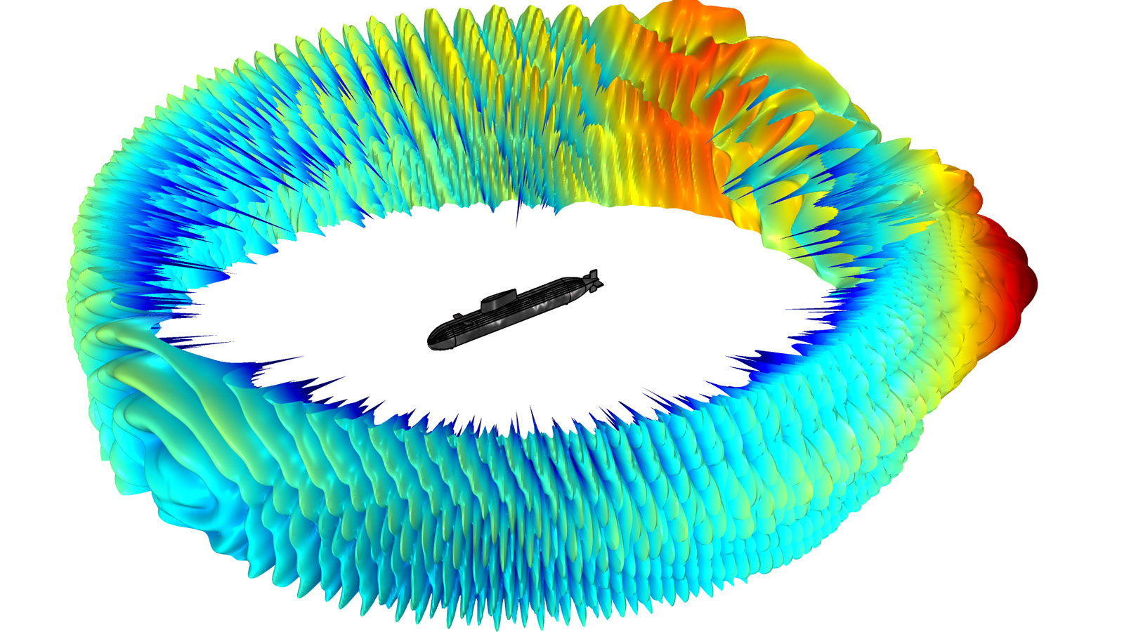
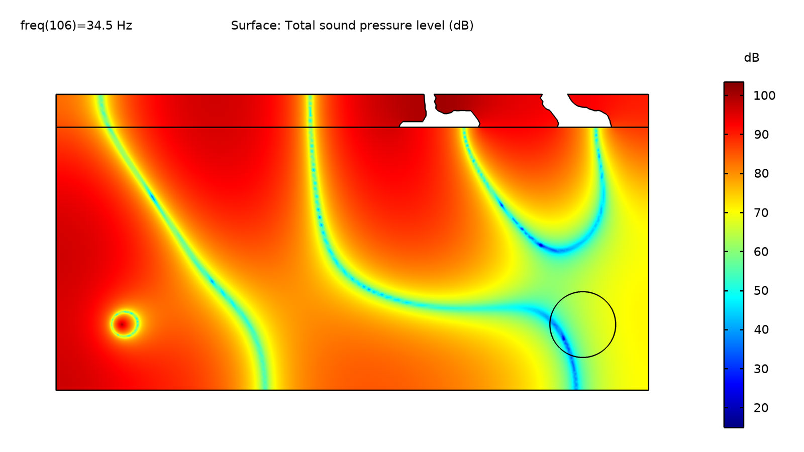
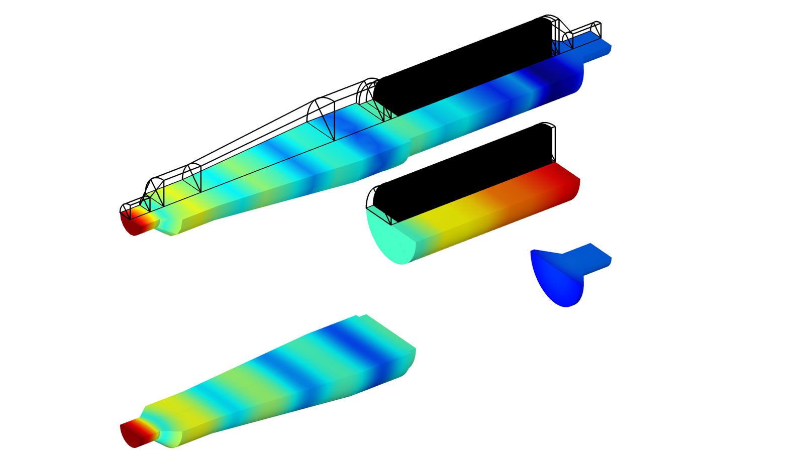
For acoustically large models, that is, models that contain many wavelengths (high frequency or large domains), you can enable a new Stabilized Formulation option to ensure efficient convergence at the cost of some additional degrees of freedom. For small to medium problems, the default formulation should be used. When the stabilized formulation is enabled, a new dedicated solver suggestion is used. As an example, consider the new Submarine Target Strength model, which requires the new stabilized formulation to converge above about 800 Hz. Solving the model at 5 kHz is also possible as seen in the image below (model solved in 5 hours using 160 GB of RAM on the fat node of a cluster). This corresponds to a model size of approximately 210 times 24 times 37 wavelengths.
More Efficient Half-Space and Infinite Baffle Modeling
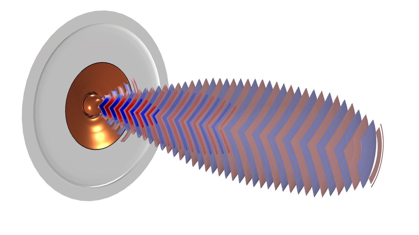
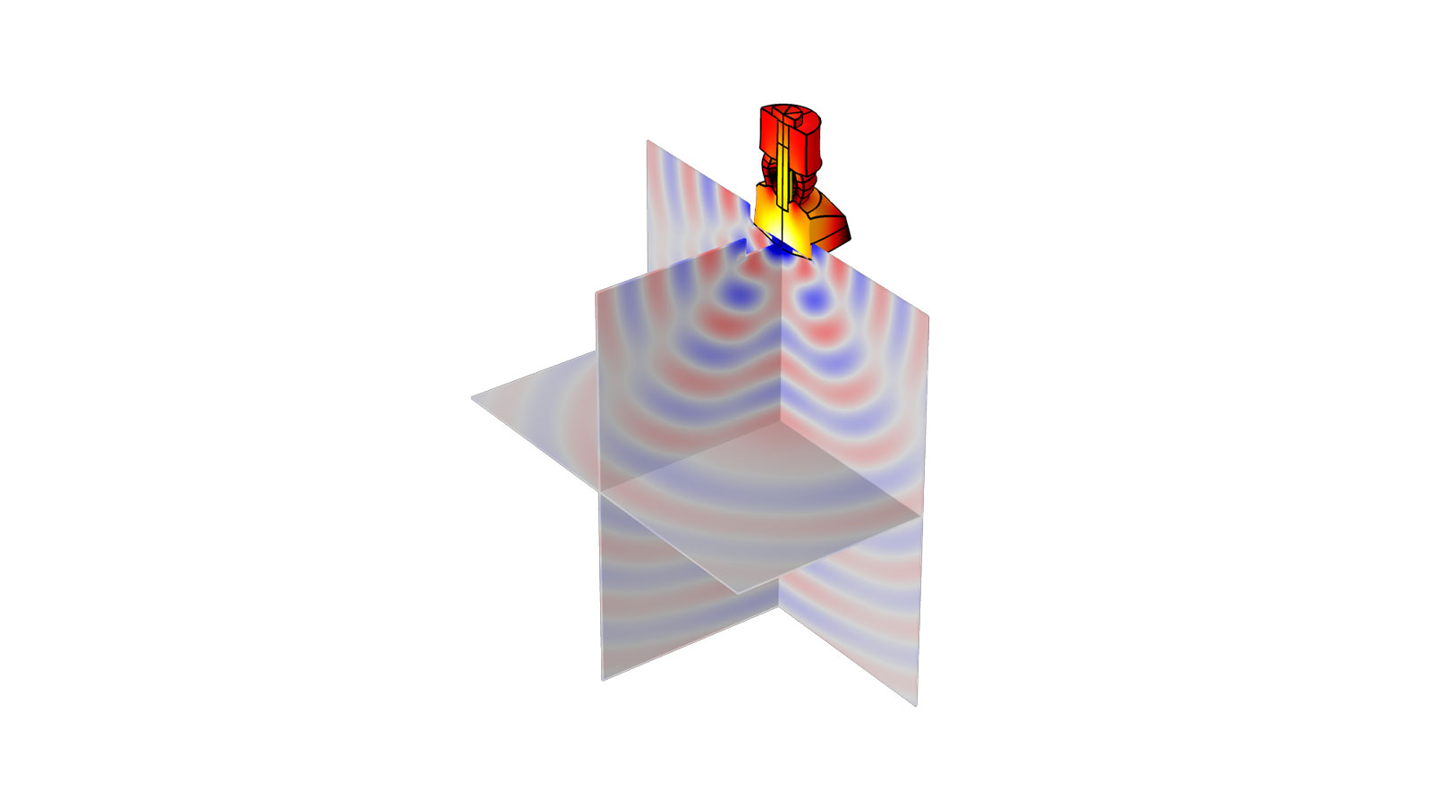
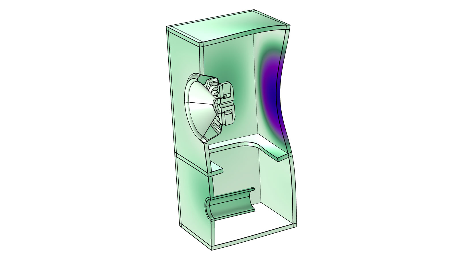
In the Pressure Acoustics, Boundary Elements interface, a new Excluded Boundary feature has been added. You can use this to exclude boundaries from the BEM model, which is particularly useful when using the Pressure Acoustics, Boundary Element interface in half-space or infinite baffle setups. In this case, all boundaries on the opposite side of the Symmetry/Infinite Sound Hard Wall should be excluded. The approach is demonstrated in the Piezoelectric Tonpilz Transducer with a Prestressed Bolt tutorial model.
Moist Air Material Generated from Thermodynamics
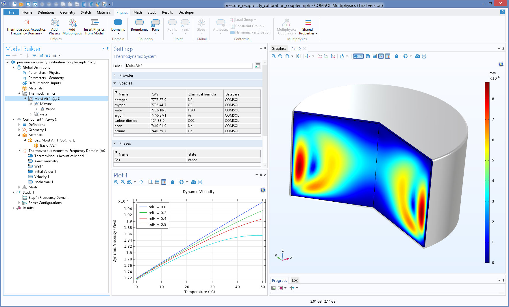
In high-fidelity and detailed absolute value acoustics simulations, it is necessary to know the material properties of moist air as a function of ambient pressure, ambient temperature, and relative humidity. Defining moist air is now possible using the predefined system for Moist Air in the Thermodynamics node. This functionality is available with the new Liquid & Gas Properties Module. One application is for the prediction of acoustic transfer impedance used in the procedure for reciprocity calibration of microphones. This is demonstrated in the Pressure Reciprocity Calibration Coupler with Detailed Moist Air Material Properties tutorial model.
Thermoviscous Boundary Layer Impedance Boundary Condition
In the Pressure Acoustics, Frequency Domain interface, the new Thermoviscous Boundary Layer Impedance boundary condition adds losses due to thermal and viscous dissipation in the acoustic boundary layers at a wall. The condition is sometimes known simply as the BLI model. The losses are included in a locally homogenized manner, where they are integrated through the boundary layers analytically. The condition is applicable in cases where boundary layers are not overlapping. Formulated differently, it is not applicable in very narrow waveguides (with dimensions comparable to the boundary layer thickness) or on highly curved boundaries. Other than that, there are no restrictions on the shape of the geometry. The method is accurate when compared to the full thermoviscous formulation (if the conditions are met) and it is much less computationally intensive. The Thermoviscous Boundary Layer Impedance boundary condition represents an engineering tool in pressure acoustics, comparable to the Narrow Region Acoustics feature. Applications are in the field of metamaterials, where the thermoviscous losses need to be included in an efficient manner to get physically correct results, but also in microacoustics in general, when modeling mobile devices, or measurement equipment. You can see this new feature in these updated tutorial models:
Performance Improvements for the Time Explicit Interfaces
The time explicit physics interfaces, which use the discontinuous Galerkin formulation (dG-FEM), benefit from a variety of performance improvements. There is a general speedup of up to 30% when solving 3D models with the Pressure Acoustics, Convected Wave Equation and the Elastic Waves, Time Explicit interfaces. As an example, the Ultrasound Flowmeter with Generic Time-of-Flight Configuration now solves in 35 min and 12 s in COMSOL Multiphysics® version 5.6 as compared to 53 min and 4 s in version 5.5, on the same standard workstation hardware. Reformulation of the Pressure Acoustics, Time Explicit interface for 2D and 2D axisymmetry reduces the number of degrees of freedom (DOFs) solved for with up to 25%. This translates into a similar reduction in memory usage and running time. The time explicit dG-FEM method has been extended to work for all mesh types, which allows the use of a structured mesh in thin elastic structures. In general, using a structured mesh gives both memory reduction and speedup. This can be seen in the Ground Motion After Seismic Event: Scattering off a Small Mountain tutorial model that now uses a quad mesh instead of triangles.
Combine Time Explicit Interfaces with ODEs
The time explicit interfaces can now be solved in combination with systems of ordinary differential equations (ODEs). This can, for example, be used to formulate user-defined frequency-dependent impedance boundary conditions in acoustics. The frequency dependency is approximated by an appropriate system of ODEs. Another useful application of ODEs is to integrate the velocity field over time in order to postprocess the displacements that result from using the Elastic Waves, Time Explicit interface. This is shown in the Isotropic-Anisotropic Sample: Elastic Wave Propagation tutorial model. Additionally, the time explicit interfaces can now be solved in combination with an algebraic equation (an equation with no time derivatives).
Axisymmetric Elastic Waves Interface and Stress, Strain, and Energy Variables
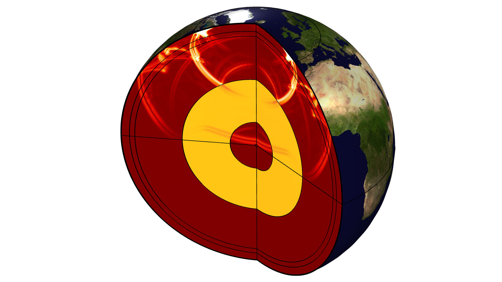
The Elastic Waves, Time Explicit interface is now available as a 2D axisymmetric formulation; an example of this is seen in the Propagation of Seismic Waves Through Earth tutorial. Additional postprocessing variables have also been added to the Elastic Waves, Time Explicit interface including volumetric and deviatoric parts of the stress and strain variables, stress and strain invariants, and energy density and energy flow variables.
Faster and Easier-to-Use Impulse Response for Ray Acoustics
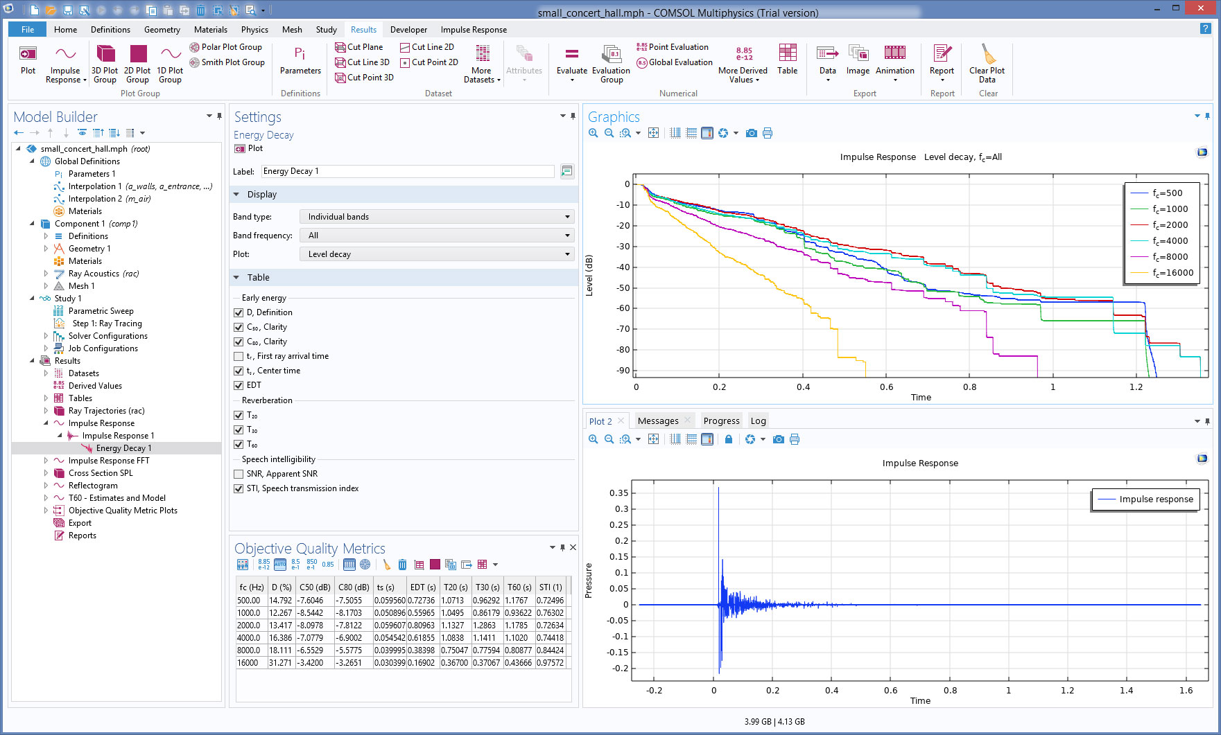
In the Ray Acoustics interface, rendering and computation time for impulse response have been greatly improved. The steps to set up impulse response are simpler and more consistent. You can analyze and compute qualitative room acoustic metrics like clarity, definition, and reverberation time based on the computed impulse response. This is done using a new Energy Decay subfeature that can be added to an Impulse Response plot. In addition, you can export the computed impulse response signal to the waveform audio file format (.wav) for further analysis. The filter kernel functionality has been improved for impulse response computation, including user-specified definition of the filter kernel and visualization of the filters.
As an example of the performance improvements, rendering the impulse response in the Small Concert Hall Acoustics tutorial model (using 20,000 rays and 6 octave bands) has reduced by nearly a factor 8, from 8 min in COMSOL Multiphysics® version 5.5, to 1 min 10 s in version 5.6, using the same standard workstation hardware and the best practices for model setup. The speedup is even more significant when solving for a larger number of rays. In addition to faster rendering, the solution time for the impulse response models has been reduced from 4 min 40 s in version 5.5, to 3 min 30 s in version 5.6. Ray data in the Impulse Response plot now uses cached storage, which ensures fast rendering times when changing options in the impulse response plot. Once the plot is processed, upon first run, postprocessing operations such as FFT, changing filter options, or analyzing the energy decay with the new Energy Decay subfeature, happens nearly instantaneously.
There are important improvements with respect to impulse response analysis, as well as new functionality, for the Energy Decay subfeature. This includes more precise computation of arrival time at the receiver when the source or the last reflection is close to the receiver. Direct sound now gets a consistent arrival time computation and summation of power. To get full advantage of the new functionality, models built in earlier versions need to be updated manually. The new qualitative room acoustic metrics, available when using the Energy Decay subfeature, are: reverberation times (T20, T30, and T60), clarity, definition, EDT, speech transmission index (STI), and the modulation transfer functions.
Export to .WAV File Format
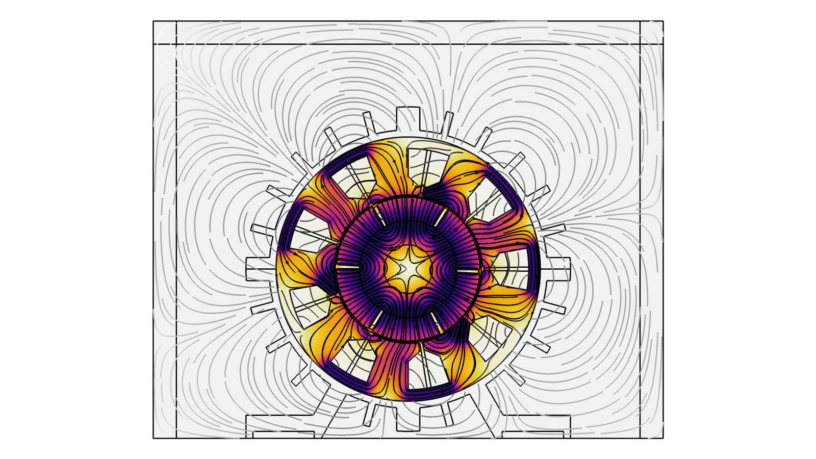
You can now export all 1D plots to .wav file format. This is particularly useful for acoustics results from a transient simulation or the impulse response in a ray acoustics simulation. Listen to the file or use it for further analysis in an external sound analysis tool. As an example, the noise of an electric motor as the RPM increases, can be played below. The example is from the new Electric Motor Noise: Analysis of a Permanent Magnet Synchronous Motor tutorial model.
News for Acoustic Port Conditions
When the Numeric (plane wave) option is used in the Port feature in a Thermoviscous Acoustics, Frequency Domain model, it now automatically detects the boundary conditions applied on the adjacent waveguide boundaries. The conditions are then automatically included when computing the mode shape of the propagating acoustic mode. This ensures physically consistent mode shapes for the port. The Numeric (plane wave) option supports the use of Wall, No Slip, Isothermal, Adiabatic, and Symmetry conditions. When generating the default solver for a setup that uses the numeric ports, the solver is now automatically configured.
In pressure acoustics, a new option has been added to compute the mode shape and cutoff frequency for numeric modes in lossless systems. For a model without any losses, the new Computed lossless mode cutoff frequency option makes it possible to run a frequency sweep using a single Boundary Mode Analysis study for each port. The port features in Pressure Acoustics, Frequency Domain and Thermoviscous Acoustics, Frequency Domain now have the option to use power scaling for mode shapes. The default is to use amplitude scaling. With the power scaling option, the computed scattering parameters can be directly related to the power carried by a specific mode.
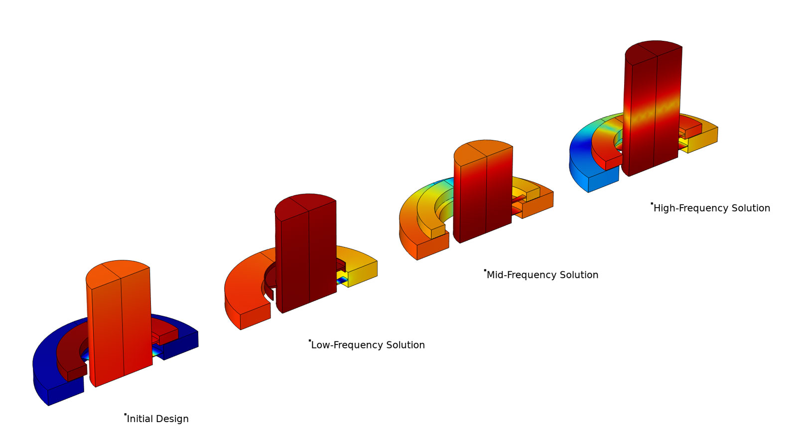
The predefined power variables of the Port boundary conditions have been reformulated such that they can be used directly in optimization models. For an example, see the Shape Optimization of an Acoustic Demultiplexer tutorial model.
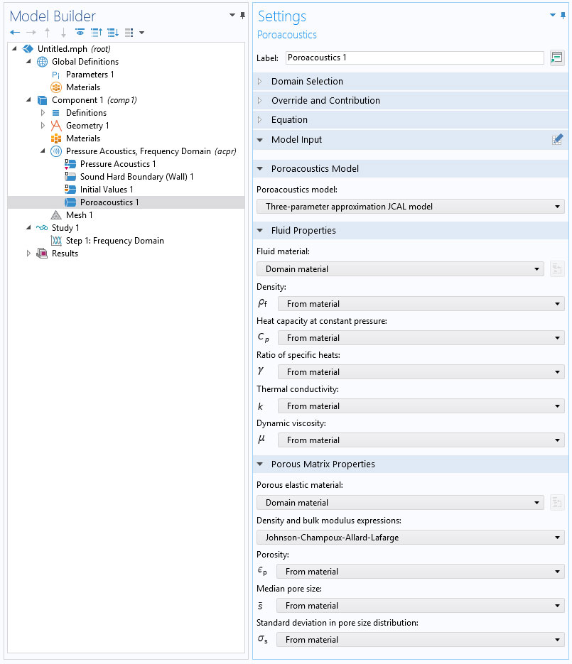
New Three-Parameter Approximation JCAL Poroacoustic Model in Poroacoustics
A new Three-parameter approximation JCAL model option has been added to the Poroacoustic feature in the Pressure Acoustics, Frequency Domain interface. The model is an approximation of the existing Johnson-Champoux-Allard-Lafarge (JCAL) model but only requires three porous parameters to be specified. The three parameters are the Porosity, the Median pore size, and the Standard deviation in pore size distribution. The model thus requires fewer inputs to define the porous matrix and the inputs in the model rely on averaged pore topology properties.
Improved Stabilization for Linearized Navier-Stokes
The stabilization in the Linearized Navier-Stokes physics interfaces has been improved with a more consistent formulation. Specifically, the balance between the stabilization contributions of the continuity, momentum, and energy equations has been improved. You can see this demonstrated in the Helmholtz Resonator with Flow: Interaction of Flow and Acoustics tutorial model, where results are smoother in the new version.
Solver Suggestions for Domain Decomposition and Shifted Laplace Methods
For pure Pressure Acoustics, Frequency Domain models, two new iterative solver suggestions have been added: one that uses the Shifted Laplace approach and another that uses Domain Decomposition. The iterative solver suggestions now automatically adds the necessary equation contributions on domains and at interior boundaries, between domains, to ensure solver efficiency. The Shifted Laplace solver is efficient for solving large models on a single machine with a lot of RAM while the Domain Decomposition method is suited for solving very large problems using distributed computation on a cluster. You can see this new functionality demonstrated in the Car Cabin Acoustics - Frequency Domain Analysis tutorial model.

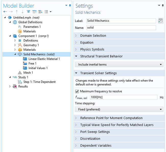
New Settings for Solving Transient Elastic Wave Problems with Solid Mechanics
New settings have been introduced in the Solid Mechanics interface that ensure a correct and efficient solver setup when solving elastic wave problems in the time domain. The settings are similar to the existing settings in the transient acoustics interfaces. In the Solid Mechanics interface node, a new Transient Solver Settings section has been introduced with an option to specify the Maximum frequency to resolve. This should be the maximum frequency content of the source's excitation or the maximum eigenmode frequency that can be excited. The automatically generated solver suggestion will have settings that use an appropriate solver method for wave propagation and ensure proper resolution in both time and space.
Faster and More Accurate Ray Rendering
When rendering a Ray Trajectories plot, a new setting can be used to accurately render all intersection points of rays with surfaces in the geometry, even if they do not correspond to output time steps in the solution data. To perfectly render every intersection point of every ray with a surface, the old implementations scaled quadratically with the number of rays, whereas the new behavior scales linearly with the number of rays, potentially giving a massive speedup when the number of rays is very large. This also applies to the calculation of intersection points between rays and a sphere, hemisphere, or plane.
New Cone-Based Ray Release: Flat Cone in 3D
In 3D models, when you release a cone of rays, you can now choose to define a ray fan or a flat cone. You can orient the flattened cone of rays so that it lies in any plane. Additionally, some other conical ray release features offer more flexibility in choosing the transverse direction, meaning that you now have more control over the exact placement of rays in the conical distribution.
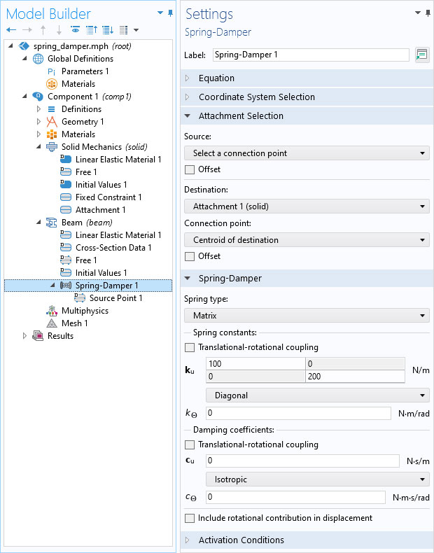
Springs and Dampers Connecting Points
In all structural mechanics interfaces, a new feature called Spring-Damper has been added to connect two points with a spring and/or damper. The points can be geometrical points, but they can also be abstract, for example, through the use of attachments or direct connections to rigid bodies. The spring can either be physical, with a force acting along the line between the two points, or described by a full matrix, connecting all translational and rotational degrees of freedom in the two points. The feature also makes it possible to connect a spring between points in two different physics interfaces.
More Flexible Licensing for Pipe Acoustics
The Pipe Acoustics, Frequency Domain and Pipe Acoustics, Transient interfaces are now available with either the Pipe Flow Module or the Acoustics Module.
Additional Important Enhancements and Updates in the Acoustics Module
- Predefined postprocessing variables are now available for the effective speed of sound magnitude and principle directions for Anisotropic Acoustics.
- Intensity variables for the scattered field formulation are now computed: background, scattered, and total field variables.
- In the Acoustic Diffusion Equation interface, the usability when importing tables defining properties in frequency bands has been improved.
- The Background Fluid Flow Coupling multiphysics feature now supports High Mach Number Flow interfaces as the source for the flow data.
New and Updated Tutorial Models and Applications
COMSOL Multiphysics® version 5.6 brings several new and updated tutorial models and applications to the Acoustics Module.
Propagation of Seismic Waves Through Earth
Application Library Title:
seismic_waves_earth
Submarine Target Strength
Application Library Title:
submarine_target_strength
Mechanical Multiport System: Elastic Wave Propagation in a Small Aluminum Plate
Application Library Title:
mechanical_multiport_system
High-Intensity Focused Ultrasound (HIFU) Propagation Through a Tissue Phantom
Application Library Title:
hifu_tissue_sample
Electric Motor Noise: Analysis of a Permanent Magnet Synchronous Motor
Application Library Title:
electric_motor_noise_pmsm
Nonlinear Slit Resonator
Application Library Title:
nonlinear_slit_resonator
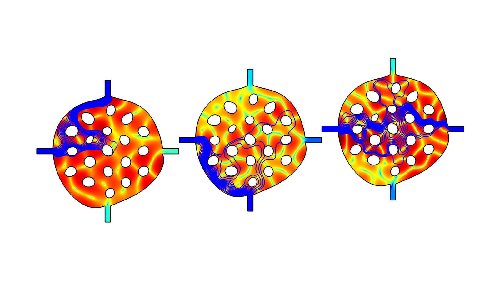
Topology Optimization and Verification of an Acoustic Mode in a Room
Application Library Title:
topology_optimization_2d_room
Nonlinear Propagation of a Cylindrical Wave — Verification Model
Application Library Title:
nonlinear_cylindrical_wave
Piezoelectric MEMS Speaker

Application Library Title:
piezo_mems_speaker
Pressure Reciprocity Calibration Coupler with Detailed Moist Air Material Properties

Application Library Title:
pressure_reciprocity_calibration_coupler
Loudspeaker Driver - Frequency Domain Analysis
Application Library Title:
loudspeaker_driver
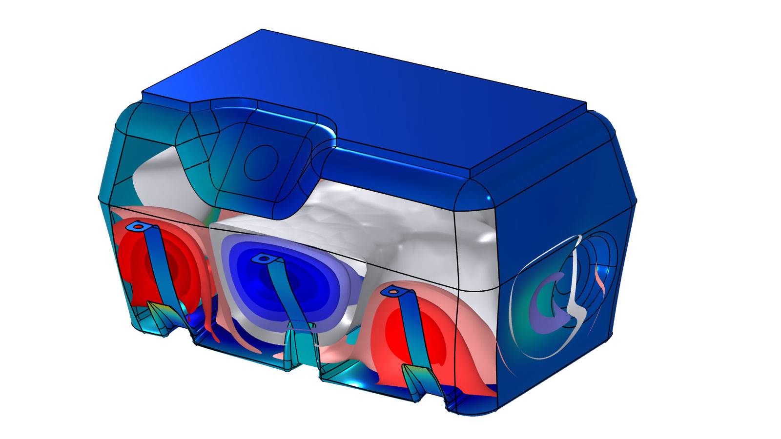
Vented Loudspeaker Enclosure
Application Library Title:
vented_loudspeaker_enclosure
Piezoelectric Tonpilz Transducer with a Prestressed Bolt
Application Library Title:
tonpilz_transducer_prestressed
The Brüel & Kjær 4134 Condenser Microphone
Application Library Title:
bk_4134_microphone
Diesel Particulate Filter Analysis Using an Acoustic Transfer Matrix
Acoustic Analysis of Leaks Around an Earbud
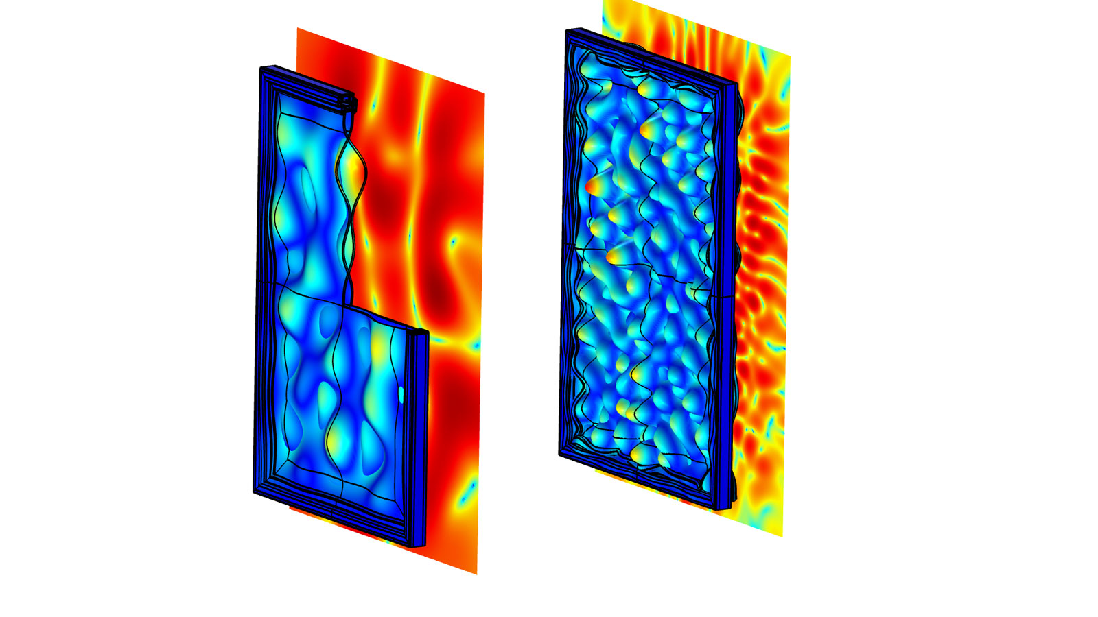
Sound Transmission Loss Through a Window
Ear Canal Acoustics
Ear Canal Simulator Optimization
Underground-Train-Induced Noise in Urban Buildings

Fuel Tank Vibration
Shape Optimization of an Acoustic Demultiplexer with 4 Ports
Application Library Title:
demultiplexer_shape_optimization
Damping Pad with a Constrained Layer
Tweeter Dome and Waveguide Shape Optimization