Particle Tracing Module
New App: Charge Exchange Cell Simulator
A charge exchange cell consists of a region of gas at an elevated pressure within a vacuum chamber. When an ion beam interacts with the higher-density gas, the ions undergo charge exchange reactions with the gas, creating energetic neutral particles. It is likely that only a fraction of the beam ions will undergo charge exchange reactions. Therefore, in order to neutralize the beam, a pair of charged deflecting plates are positioned outside the cell. In this way, an energetic neutral source can be produced.
The Charge Exchange Cell Simulator app simulates the interaction of a proton beam with a charge exchange cell containing neutral argon. User input includes several geometric parameters for the gas cell and vacuum chamber, beam properties, and the properties of the charged plates that are used to deflect the remaining ions.
The simulation app computes the efficiency of the charge exchange cell, measured as the fraction of ions that are neutralized, and records statistics about the different types of collisions that occur.
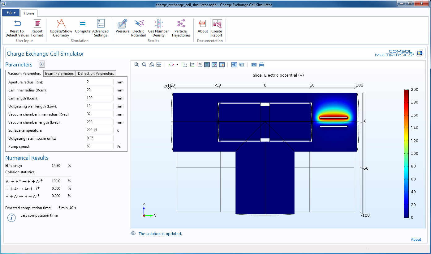 User interface for the Charge Exchange Cell Simulator app.
New App: Laminar Static Particle Mixer Designer
In static mixers, a fluid is pumped through a pipe containing stationary mixing blades. This mixing technique is well suited for laminar flow mixing, because it generates only small pressure losses in this flow regime. When a fluid is pumped through the channel, the alternating directions of the cross-sectional blades mix the fluid as it passes along the length of the channel. The static mixing technique allows for precise control over the amount of mixing that takes place throughout the process. However, the performance of the mixer can vary greatly, depending on its geometry.
The Laminar Static Particle Mixer Designer app computes the fluid velocity and pressure field in a static mixer, as well as the trajectories of particles that are carried by the fluid. Because the particles have mass, they do not follow the fluid velocity streamlines exactly, causing some particles to hit the mixing blades.
The example app computes the transmission probability of particles in the mixer. It also evaluates the index of dispersion, which is a measurement of the uniformity with which different species of particles are mixed together.
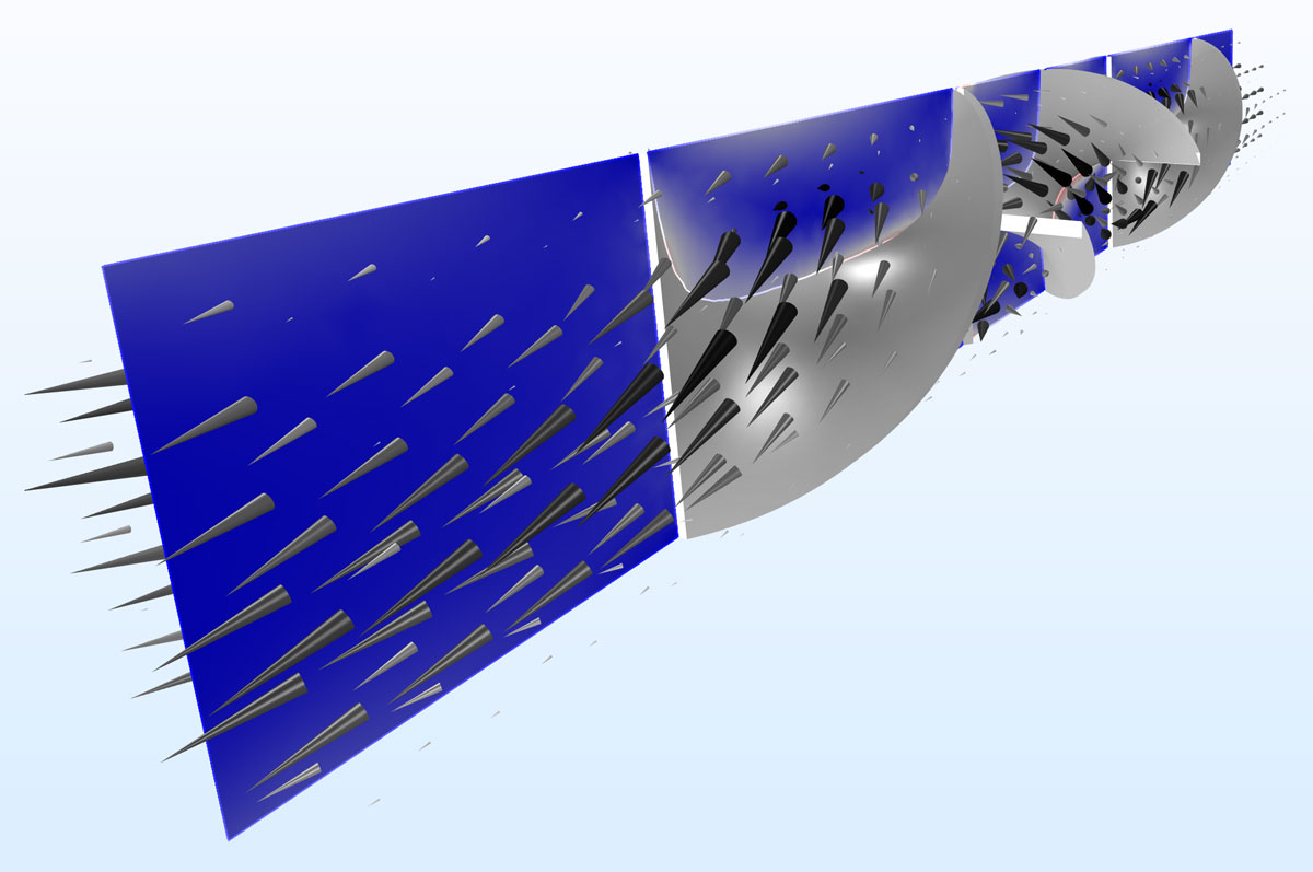 Fluid velocity field in the laminar static mixer (arrows) and shear rate in a cross section (slice plot).
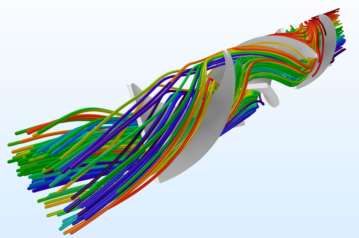 Particle trajectories in the laminar static mixer. To visualize the mixer performance more easily, only a fraction of the particles are rendered and they are colored according to their initial positions.
Release from Edges and Points
With COMSOL Multiphysics version 5.2, the Release from Edge and Release from Point nodes can be used to release particles from edges and points in a geometry, respectively. When releasing particles along an edge, the particle positions can be mesh-based, weighted by a user-defined density function, or uniformly distributed along the edge length.
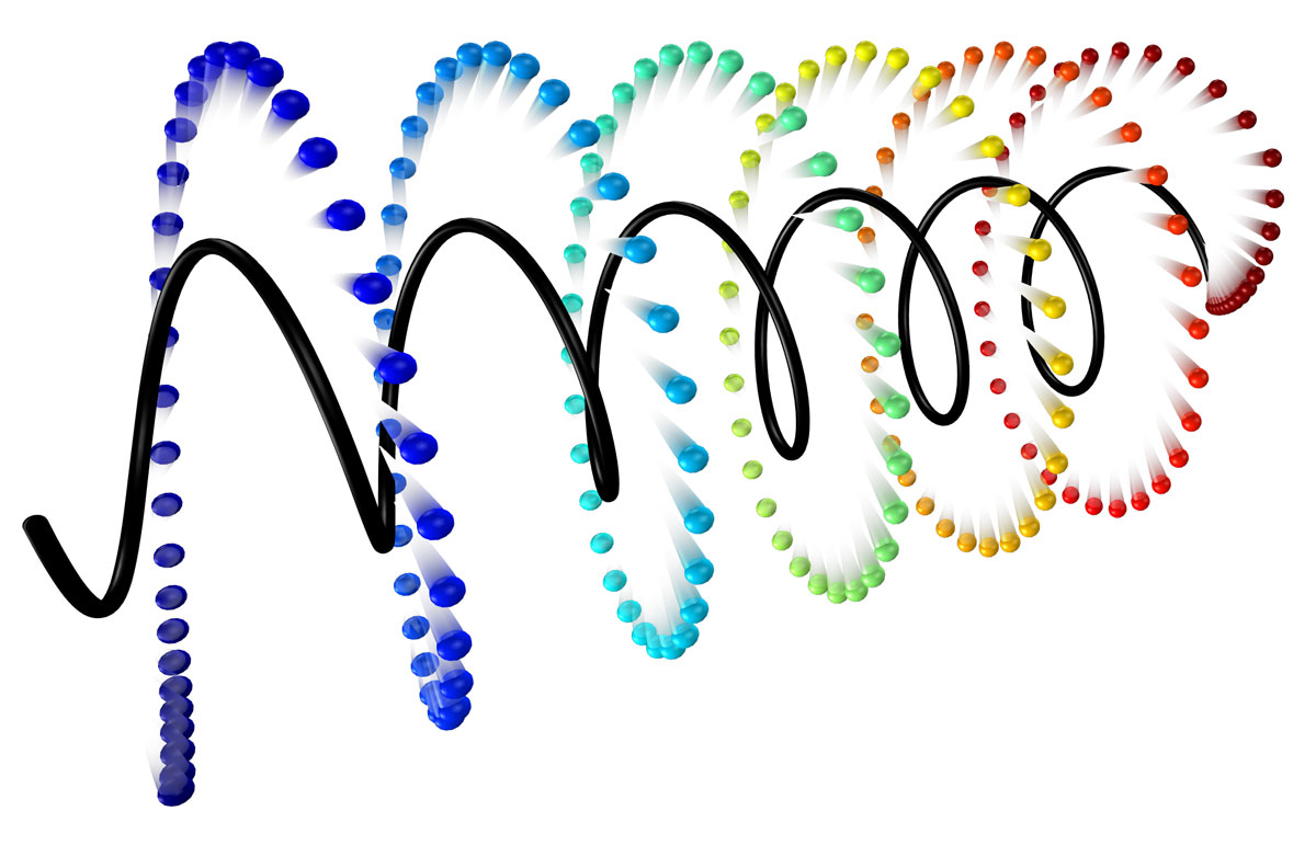 It is possible to release particles along an arbitrary curve, such as the helix shown above.
Improved Density-Based Release
The release features that initialize particle position according to a density function have new settings that make them much more accurate. It is now possible to specify a Release distribution accuracy order and Position refinement factor in the settings for the Release, Inlet, and Particle Beam nodes as well as the new Release from Edge node. The improvement in accuracy is most noticeable when the underlying mesh is very coarse or the particle density varies significantly across different mesh elements.
Particles are released on a coarse mesh with a Gaussian distribution of initial coordinates. The distribution of particle positions more closely matches the specified distribution when the Position refinement factor is 10 (red) than when it is 0 (blue).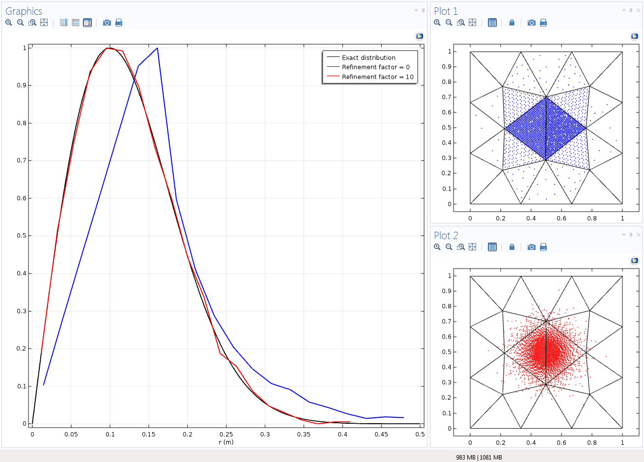
Particles are released on a coarse mesh with a Gaussian distribution of initial coordinates. The distribution of particle positions more closely matches the specified distribution when the Position refinement factor is 10 (red) than when it is 0 (blue).
Charge Exchange Collisions
You can now add two new collision types to the Collisions node: Resonant Charge Exchange and Nonresonant Charge Exchange.
The Resonant Charge Exchange node is used when energetic ions undergo charge exchange reactions with ambient neutral atoms of the same element or molecules of the same substance. The Nonresonant Charge Exchange feature is used when the ionized and neutral species are of different elements or substances. In both cases, after the collision, it is possible to continue tracking the ionized species, neutral species, or both.
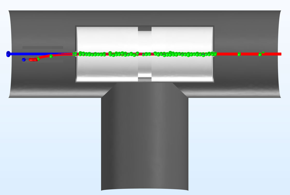 In a charge exchange cell, an energetic proton beam (red) propagates through a gas cell (light gray) that is maintained at a higher pressure than its surroundings. The resulting charge exchange collisions create fast, neutral hydrogen (blue) and slow-moving argon ions (green).
Particle Beam Improvements
New options are available in the Particle Beam feature to make the transverse position and velocity distributions easier to specify. This makes it much easier to release beams with phase space ellipses of a certain size, shape, and orientation. The equation display has been improved and augmented with images to provide a better indication of what the various options do.
| Sampling | Orientation | Velocity Specification | Image |
|---|---|---|---|
| Uniform | Upright | Twiss parameters | 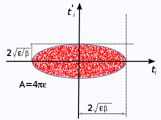 |
| Uniform | Not upright | Twiss parameters | 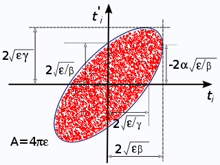 |
| Uniform | Upright | Ellipse dimensions | 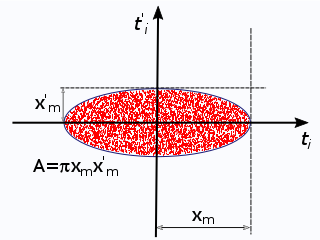 |
| Uniform | Not upright | Ellipse dimensions | 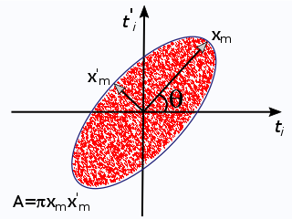 |
| Gaussian | Upright | Twiss parameters | 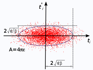 |
| Gaussian | Upright | Twiss parameters | 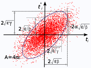 |
| Gaussian | Upright | Ellipse dimensions | 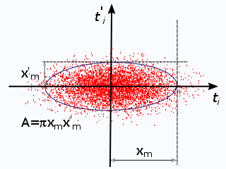 |
| Gaussian | Not upright | Ellipse dimensions | 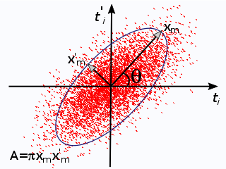 |
Particle Counters
A Particle Counter feature is a domain or boundary feature that provides information about particles arriving on a set of selected domains or surfaces from a release feature. Such quantities include the number of particles transmitted, transmission probability, transmitted current, mass flow rate, and more. This feature, new with COMSOL Multiphysics version 5.2, provides convenient results expressions that can be used in the Filters node of the Particle Trajectories plot, which allows only the particles that reach the particle counter selection to be visualized.
The following variables are provided by the Particle Counter feature, with the feature tag <tag>:
<tag>.Nfin- The number of transmitted particles from the release feature to the particle counter at the final time.
<tag>.Nsel- The number of transmitted particles from the release feature to the particle counter.
<tag>.alpha- The transmission probability from the release feature to the particle counter.
<tag>.rL- A logical expression for particle inclusion. This can be set in the Filter node of the Particle Trajectories plot in order to visualize the particles that connect the release feature to the counter.
<tag>.It- The transmitted current from the release feature to the particle counter. This variable is only available for the Charged Particle Tracing interface when the particle release specification is set to Specify current.
<tag>.mdott- The transmitted mass flow rate from the release feature to the particle counter. This variable is only available for the Particle Tracing for Fluid Flow interface when the particle release specification is set to Specify mass flow rate.
If the Particle Counter feature is a Particle Beam feature in the Charged Particle Tracing interface, additional variables for the average position, velocity, and energy of the transmitted particles are available.
Particle-Matter Interactions
You can now model the interaction of energetic ions with solid matter using the dedicated Particle-Matter Interactions feature. This feature supports two subfeatures for different types of interactions:
- Ionization loss is used to model the continuous loss of energy as ions interact with electrons in the target material.
- Nuclear stopping is used to model the deflection of energetic ions by target nuclei.
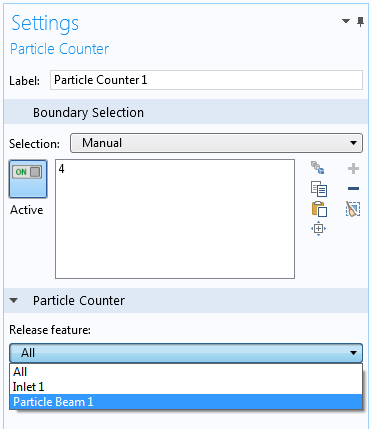
 As the initial kinetic energy of ions is increased, their interaction with solid material becomes dominated by ionization loss instead of stochastic nuclear interactions. As a consequence, highly energetic ions tend to follow nearly straight paths, whereas less energetic ions follow more random paths.
New Tutorial: Ion Range Benchmark
The Ion Range Benchmark model simulates the passage of energetic protons through silicon with both ionization losses and nuclear scattering. The initial energy of the protons is varied using a parametric sweep from 1 keV to 100 MeV.
The average path length of the protons is compared to published values of the ion range under the continuous slowing down approximation (CSDA) as well as the projected range in the initial direction of motion. Simulated and experimental data agree well.
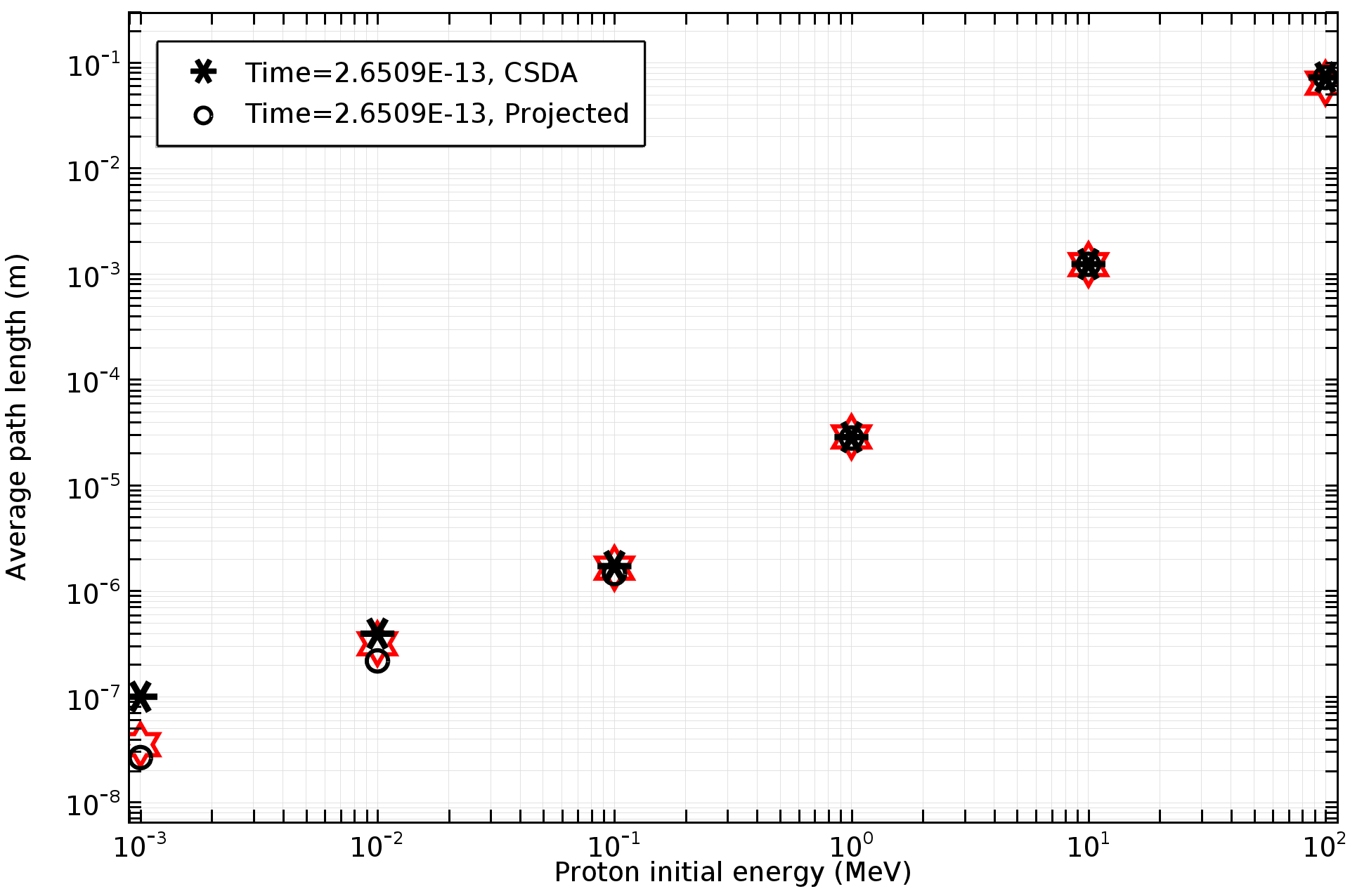 Comparison of computed path length (red) to experimental measurements of the ion range under the continuous slowing down approximation (CSDA) and the projected range.
New Tutorial: Sensitive High-Resolution Ion Microprobe (SHRIMP)
The Sensitive High-Resolution Ion Microprobe (SHRIMP) is used to transmit ions of a given initial energy and specified charge-to-mass ratio by subjecting an incoming beam to appropriately tuned electric and magnetic forces. The beam is first sent through a curved sector with a radial electric force, then through a second curved sector with a uniform magnetic flux density.
This tutorial model utilizes the Particle Beam feature of the COMSOL Multiphysics® software to examine the performance of the high-precision spectrometer, where only a fraction of the incoming beam is transmitted to the detector. The model calculates the transmission probability and visualizes the nominal trajectory of the transmitted beam.
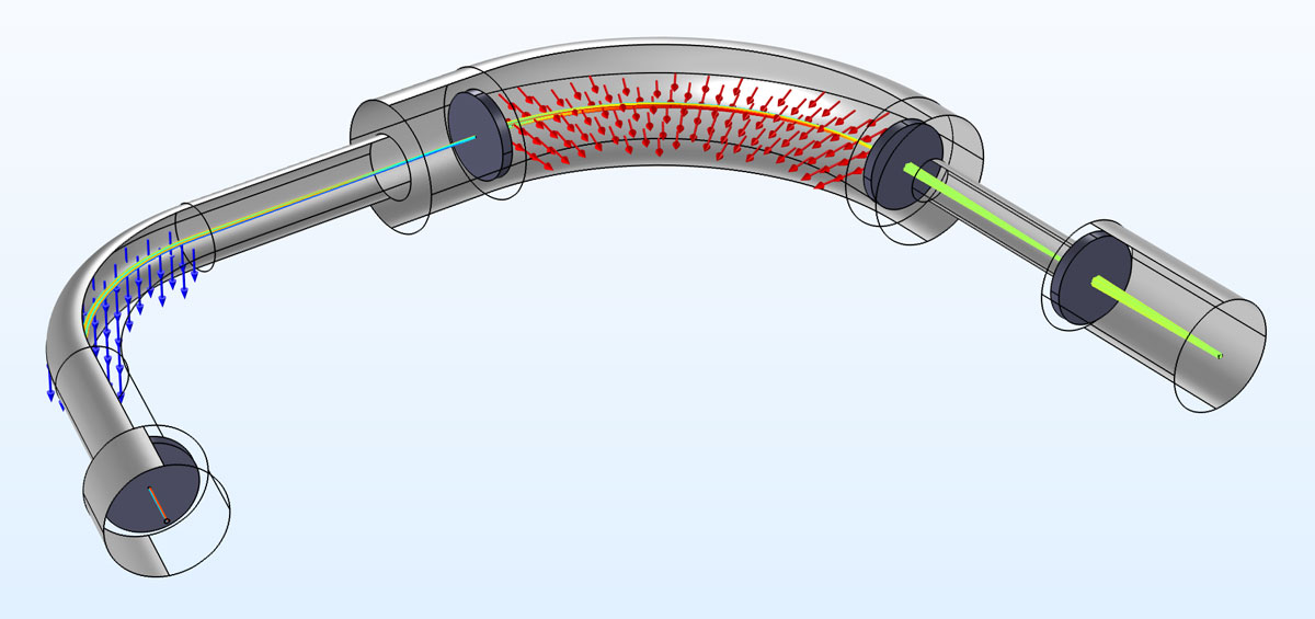 An ion beam in the SHRIMP is subjected to a radial electric field (red) followed by a uniform magnetic flux density (blue). The color of the beam indicates the particle velocity norm.