Technical Papers and Presentations

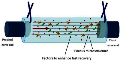
Biodegradable scaffolds are often inserted in the body, to provide mechanical support to recovering broken or damaged tissues. Monitoring the degradation chemistry and mechanical response of these scaffolds is important: their degradation rate should match tissue regeneration rate, while providing sufficient mechanical support. This requires a thorough study of the complex coupling between the degradation chemistry and the mechanical and transport properties of the scaffold. In this study, we present a formulation intended provide a predictive framework for studying the degradation chemistry and the corresponding evolution of properties of scaffolds. We choose a 3-component system, or ‘mixture’ for our analysis - comprising of the degrading solid (scaffold), the product of degradation (called the monomeric fluid) and a stimulant base fluid like water.

The model problem involves 8 variables: volume fractions (or concentrations) of the three components, displacement of the solid, velocities of the three components and the pressure in the system. Our mixture theoretic formulation consists of equations for the balance of mass and momentum for the components and the mixture, along with appropriate constitutive equations and a ‘saturation constraint’ for the mixture.

The formulation leads to transient nonlinear differential-algebraic equations, which have been implemented in COMSOL Multiphysics^® simulation software. We used the Weak Form PDE interface for analysis of our numerical framework. Numerical experiments were carried out using the Method of Manufactured Solutions [1], on a 2D domain. The planar domain was uniformly discretized into quadrilateral elements and piecewise Lagrange polynomials have been implemented as shape functions. For the time-stepping, we used the backward difference formula (BDF), configuring it to allow orders 2-5 and flexible time step sizes. We also enforced a fixed maximum time step size for all the simulations.

In order to study the stability of the numerical scheme, simulations were performed over different ranges of solid and fluid volume fraction values. Also, convergence analysis of the numerical scheme was done by performing a parametric sweep over different refinement levels. The global errors were estimated using the ‘Integration’ operator within the ‘Component Couplings’ feature. We observed that, barring very high solid volume fraction values, without any additional stabilization, the numerical scheme was stable when the order of interpolation for pressure was one less than that for the vector fields (solid displacement and velocities), i.e. cubic polynomials for vectors and quadratic for pressure, or quadratic for vectors and linear for pressure, with linear interpolation for volume fractions in both cases. It was observed that, over different ranges of values of volume fractions, the convergence rates (L² error norm) for the fluid velocities and volume fraction remained constant at about 2, whereas that of the solid displacement and velocity were about 3, irrespective of the interpolation order. The convergence rate of pressure, however varied according to its interpolation order – a convergence rate of about 2 and 3 was obtained for linear and quadratic pressure interpolation functions respectively.

[1] K. Salari, P. Knupp, Code verification by the method of manufactured solutions, Sandia National Laboratories, 2000.