Navier-Stokes Equations
What Are the Navier-Stokes Equations?
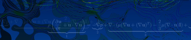
The Navier-Stokes equations govern the motion of fluids and can be seen as Newton's second law of motion for fluids. In the case of a compressible Newtonian fluid, this yields

where u is the fluid velocity, p is the fluid pressure, ρ is the fluid density, and μ is the fluid dynamic viscosity. The different terms correspond to the inertial forces (1), pressure forces (2), viscous forces (3), and the external forces applied to the fluid (4). The Navier-Stokes equations were derived by Navier, Poisson, Saint-Venant, and Stokes between 1827 and 1845.
These equations are always solved together with the continuity equation:

The Navier-Stokes equations represent the conservation of momentum, while the continuity equation represents the conservation of mass.
How Do They Apply to Simulation and Modeling?
These equations are at the heart of fluid flow modeling. Solving them, for a particular set of boundary conditions (such as inlets, outlets, and walls), predicts the fluid velocity and its pressure in a given geometry. Because of their complexity, these equations only admit a limited number of analytical solutions. It is relatively easy, for instance, to solve these equations for a flow between two parallel plates or for the flow in a circular pipe. For more complex geometries, however, the equations need to be solved.
Example: Laminar Flow Past a Backstep
In the following example, we numerically solve the Navier-Stokes equations (hereon also referred to as "NS equations") and the mass conservation equation in a computational domain. These equations need to be solved with a set of boundary conditions:
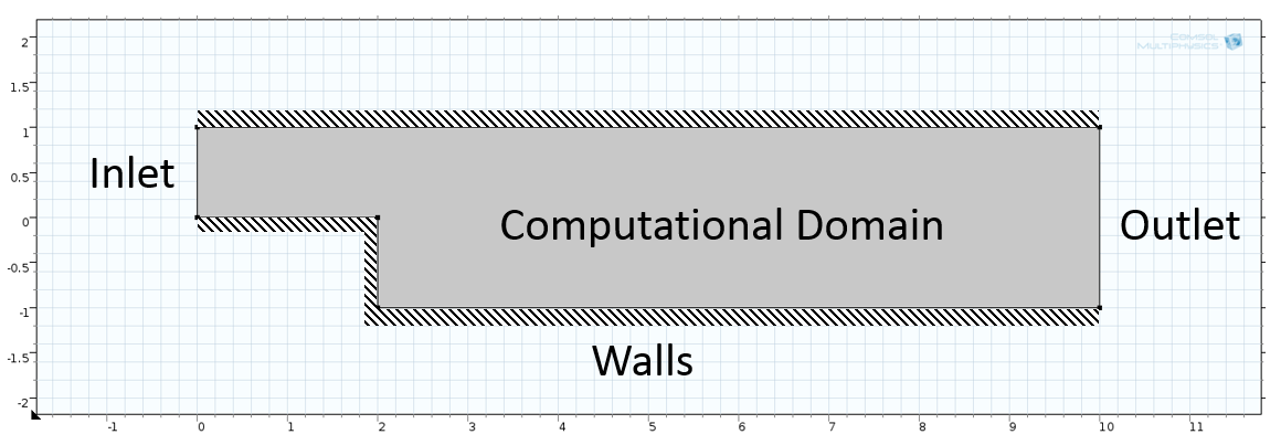
The fluid velocity is specified at the inlet and pressure prescribed at the outlet. A no-slip boundary condition (i.e., the velocity is set to zero) is specified at the walls. The numerical solution of the steady-state NS (the time-dependent derivative in (1) is set to zero) and continuity equations in the laminar regime and for constant boundary conditions is as follows:
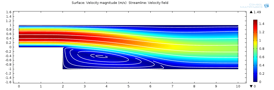 Velocity magnitude profile and streamlines.
Velocity magnitude profile and streamlines.
Velocity magnitude profile and streamlines.
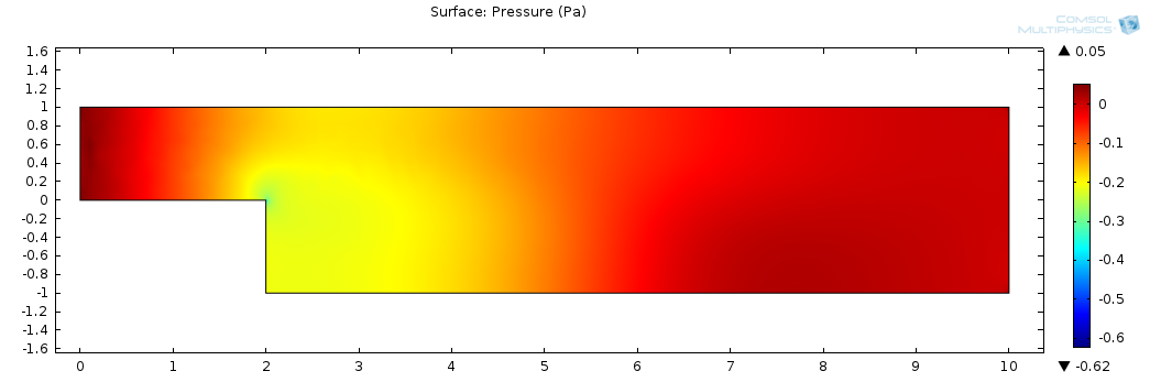 Pressure field.
Pressure field.
Pressure field.
Different Flavors of the Navier-Stokes Equations
Depending on the flow regime of interest, it is often possible to simplify these equations. In other cases, additional equations may be required. In the field of fluid dynamics, the different flow regimes are categorized using a nondimensional number, such as the Reynolds number and the Mach number.
About the Reynolds and Mach Numbers
The Reynolds number, Re=ρUL/μ, corresponds to the ratio of inertial forces (1) to viscous forces (3). It measures how turbulent the flow is. Low Reynolds number flows are laminar, while higher Reynolds number flows are turbulent.
The Mach number, M=U/c, corresponds to the ratio of the fluid velocity, U, to the speed of sound in that fluid, c. The Mach number measures the flow compressibility.
In the flow past a backstep example, Re = 100 and M = 0.001, which means that the flow is laminar and nearly incompressible. For incompressible flows, the continuity equation yields:

Because the divergence of the velocity is equal to zero, we can remove the term:

from the viscous force term in the NS equations in the case of incompressible flow.
In the following section, we examine some particular flow regimes.
Low Reynolds Number/Creeping Flow
When the Reynolds number is very small (Re≪1) , the inertial forces (1) are very small compared to the viscous forces (3) and they can be neglected when solving the NS equations. To illustrate this flow regime, we will look at pore-scale flow experiments conducted by Arturo Keller, Maria Auset, and Sanya Sirivithayapakorn of the University of California, Santa Barbara.
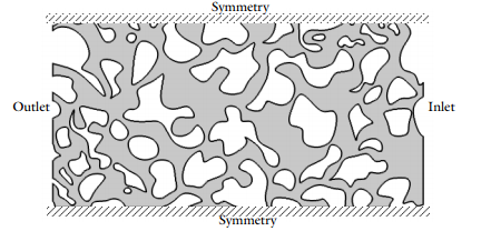 Graphic showing the boundary conditions in the pore-scale flow experiment.
Graphic showing the boundary conditions in the pore-scale flow experiment.
Graphic showing the boundary conditions in the pore-scale flow experiment.
About the Experiment
The domain of interest covers 640 μm by 320 μm. Water moves from right to left across the geometry. The flow in the pores does not penetrate the solid part (gray area in the figure above). The inlet and outlet fluid pressures are known. Since the channels are at most 0.1 millimeters in width and the maximum velocity is lower than 10-4 m/s, the maximum Reynolds number is less than 0.01. Because there are no external forces (gravity is neglected), the force term (4) is also equal to zero.
Therefore, the NS equations reduce to:

Modeling the Experiment
The below plot shows the resulting velocity contours and pressure field (height).
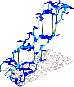
The flow is driven by a higher pressure at the inlet than at the outlet. These results show the balance between the pressure force (2) and the viscous forces (3) in the NS equations. Along the thinner channels, the impact of viscous diffusion is larger, which leads to higher pressure drops.
High Reynolds Number/Turbulent Flow
In engineering applications where the Reynolds number is very high, the inertial forces (1) are much larger than the viscous forces (3). Such turbulent flow problems are transient in nature; a mesh that is fine enough to resolve the size of the smallest eddies in the flow needs to be used.
Running such simulations using the NS equations is often beyond the computational power of most of today's computers and supercomputers. Instead, we can use a Reynolds-Averaged Navier-Stokes (RANS) formulation of the Navier-Stokes equations, which averages the velocity and pressure fields in time.
These time-averaged equations can then be computed in a stationary way on a relatively coarse mesh, thus drastically reducing the computing power and time required for such simulations (typically a few minutes for two-dimensional flow and a few minutes to a few days for three-dimensional flow).
The Reynolds-Averaged Navier-Stokes (RANS) formulation is as follows:

Here, U and P are the time-averaged velocity and pressure, respectively. The term μT represents the turbulent viscosity, i.e., the effects of the small-scale time-dependent velocity fluctuations that are not solved for by the RANS equations.
The turbulent viscosity, μT, is evaluated using turbulence models. The most common one is the k-ε turbulence model (one of many RANS turbulence models). This model is often used in industrial applications because it is both robust and computationally inexpensive. It consists of solving two additional equations for the transport of turbulent kinetic energy k and turbulent dissipation ϵ.
To illustrate this flow regime, let us look at the flow in a much larger geometry than the por-scale flow: a typical ozone purification reactor. The reactor is about 40 meters long and looks like a maze with partial walls or baffles that divide the space into room-sized compartments. Based on the inlet velocity and diameter, which in this case correspond to 0.1 m/s and 0.4 meters respectively, the Reynolds number is 400,000. This model is solved for the time-averaged velocity, U; pressure, P; turbulent kinetic energy, k; and turbulent dissipation, ϵ:
 The results show the flow patterns, flow velocity, and turbulent viscosity μT.
The results show the flow patterns, flow velocity, and turbulent viscosity μT.
The results show the flow patterns, flow velocity, and turbulent viscosity μT.
Flow Compressibility
The flow compressibility is measured by the Mach number. All the previous examples are weakly compressible, meaning that the Mach number is lower than 0.3.
Incompressible Flow
When the Mach number is very low, it is OK to assume that the flow is incompressible. This is often a good approximation for liquids, which are much less compressible than gases. In that case, the density is assumed to be constant and the continuity equation reduces to ∇⋅u=0. The creeping flow example showing water flowing at a low speed through the porous media is a good example of incompressible flow.
Compressible Flow
In some cases, the flow velocity is large enough to introduce significant changes in the density and temperature of the fluid. These changes can be neglected for M<0.3. For M>0.3, however, the coupling between the velocity, pressure, and temperature field becomes so strong that the NS and continuity equations need to be solved together with the energy equation (the equation for heat transfer in fluids). The energy equation predicts the temperature in the fluid, which is needed to compute its temperature-dependent material properties.
Compressible flow can be laminar or turbulent. In the next example, we look at a high-speed turbulent gas flow in a diffuser (a converging and diverging nozzle).
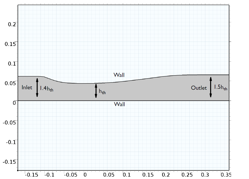
The diffuser is transonic in the sense that the flow at the inlet is subsonic, but due to the contraction and the low outlet pressure, the flow accelerates and becomes sonic (M = 1) in the throat of the nozzle.
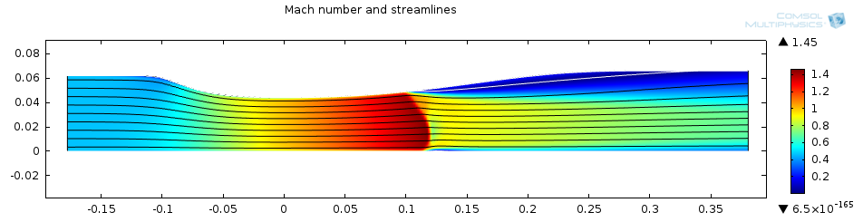
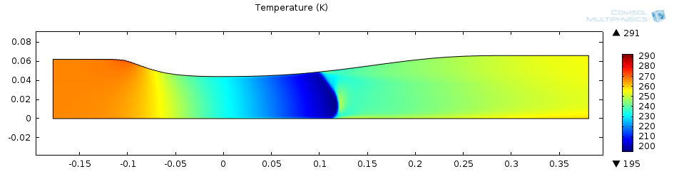
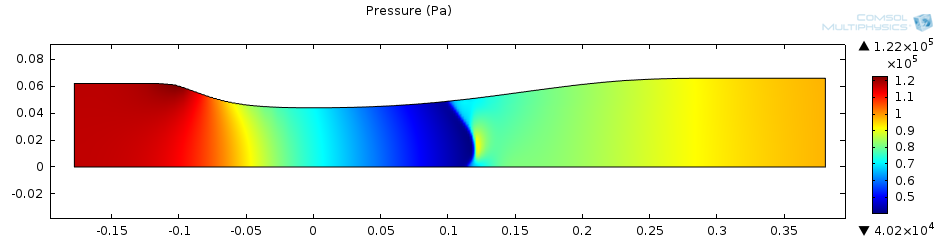
The results in these three plots show strong similarities, which confirms the strong coupling between the velocity, pressure, and temperature fields. After a short region of supersonic flow (M > 1), a normal shock wave brings the flow back to subsonic flow. This set-up has been studied in a number of experiments and numerical simulations by M. Sajben et. al. [1-6].
What Flow Regimes Cannot Be Solved by the Navier-Stokes Equations?
The Navier-Stokes equations are only valid as long as the representative physical length scale of the system is much larger than the mean free path of the molecules that make up the fluid. In that case, the fluid is referred to as a continuum. The ratio of the mean free path, λ, and the representative length scale, L, is called the Knudsen number, Kn=λ/L
The NS equations are valid for Kn<0.01. For 0.01<Kn<0.1, these equations can still be used, but they require special boundary conditions. For Kn>0.1, they are not valid. At the ambient pressure of 1 atm – for instance, the mean free path of air molecules – is 68 nanometers. The characteristic length of your model should therefore be larger than 6.8 μm for the NS equations to be valid.
Published: January 15, 2015Last modified: February 22, 2017
References
- M. Sajben, J.C. Kroutil, and C.P. Chen, “A High-Speed Schlieren Investigation of Diffuser Flows with Dynamic Distortion”, AIAA Paper 77-875, 1977.
- T.J. Bogar, M. Sajben, and J.C. Kroutil, “Characteristic Frequencies of Transonic Diffuser Flow Oscillations,” AIAA Journal, vol. 21, no. 9, pp. 1232–1240, 1983.
- J.T. Salmon, T.J. Bogar, and M. Sajben, “Laser Doppler Velocimetry in Unsteady, Separated, Transonic Flow”, AIAA Journal, vol. 21, no. 12, pp. 1690–1697, 1983.
- T. Hsieh, A.B. Wardlaw Jr., T.J. Bogar, P. Collins, and T. Coakley, “Numerical Investigation of Unsteady Inlet Flowfields,” AIAA Journal, vol. 25, no. 1, pp. 75–81, 1987.
- http://www.grc.nasa.gov/WWW/wind/valid/transdif/transdif01/transdif01.html
- http://www.grc.nasa.gov/WWW/wind/valid/transdif/transdif02/transdif02.html