Finite Element Mesh Refinement
What Is Finite Element Mesh Refinement?
Engineers and scientists use finite element analysis (FEA) software to build predictive computational models of real-world scenarios. The use of FEA software begins with a computer-aided design (CAD) model that represents the physical parts being simulated as well as knowledge of the material properties and the applied loads and constraints. This information enables the prediction of real-world behavior, often with very high levels of accuracy.
The accuracy that can be obtained from any FEA model is directly related to the finite element mesh that is used. The finite element mesh is used to subdivide the CAD model into smaller domains called elements, over which a set of equations are solved. These equations approximately represent the governing equation of interest via a set of polynomial functions defined over each element. As these elements are made smaller and smaller, as the mesh is refined, the computed solution will approach the true solution.
This process of mesh refinement is a key step in validating any finite element model and gaining confidence in the software, the model, and the results.
The Mesh Refinement Process
A good finite element analyst starts with both an understanding of the physics of the system that is to be analyzed and a complete description of the geometry of the system. This geometry is represented via a CAD model. A typical CAD model will accurately describe the shape and structure, but often also contain cosmetic features or manufacturing details that can prove to be extraneous for the purposes of finite element modeling. The analyst should put some engineering judgment into examining the CAD model and deciding if these features and details can be removed or simplified prior to meshing. Starting with a simple model and adding complexity is almost always easier than starting with a complex model and simplifying it.
The analyst should also know all of the physics that are relevant to the problem, the materials properties, the loads, the constraints, and any elements that can affect the results of interest. These inputs may have uncertainties in them. For instance, the material properties and loads may not always be precisely known. It is important to keep this in mind during the modeling process, as there is no benefit in trying to resolve a model to greater accuracy than the input data admits.
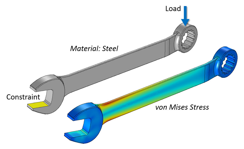 Finite element model of a wrench, including stresses.
A finite element model of a wrench and the computed stresses. The mesh is not shown.
Finite element model of a wrench, including stresses.
A finite element model of a wrench and the computed stresses. The mesh is not shown.
Once all of this information is assembled into an FEA model, the analyst can begin with a preliminary mesh. Early in the analysis process, it makes sense to start with a mesh that is as coarse as possible – a mesh with very large elements. A coarse mesh will require less computational resources to solve and, while it may give a very inaccurate solution, it can still be used as a rough verification and as a check on the applied loads and constraints.
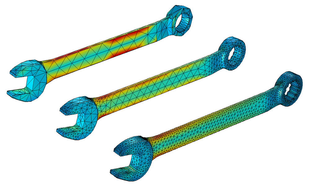 Mesh refinement study of a wrench, with a varying mesh coarseness.
The first few iterations of a mesh refinement study of a wrench, starting with a very coarse mesh.
Mesh refinement study of a wrench, with a varying mesh coarseness.
The first few iterations of a mesh refinement study of a wrench, starting with a very coarse mesh.
After computing the solution on the coarse mesh, the process of mesh refinement begins. In its simplest form, mesh refinement is the process of resolving the model with successively finer and finer meshes, comparing the results between these different meshes. This comparison can be done by analyzing the fields at one or more points in the model or by evaluating the integral of a field over some domains or boundaries.
By comparing these scalar quantities, it is possible to judge the convergence of the solution with respect to mesh refinement. After comparing a minimum of three successive solutions, an asymptotic behavior of the solution starts to emerge, and the changes in the solution between meshes become smaller. Eventually, these changes will be small enough that the analyst can consider the model to be converged. This is always a judgment call on the part of the analyst, who knows the uncertainties in the model inputs and the acceptable uncertainty in the results.
Different Mesh Refinement Metrics
Studying convergence requires choosing an appropriate mesh refinement metric. This metric can be either local or global. That is, the metric can be defined at one location in the model or as the integral of the fields over the entire model space. An example of a local metric is the displacement or stress at a point within a structural analysis. An example of a global metric is the integral of the strain energy density over all domains. Both the stresses and the strain are computed based upon the gradient of the solution and the displacement field. Gradients of the solution are always computed to one order lower polynomial approximation.
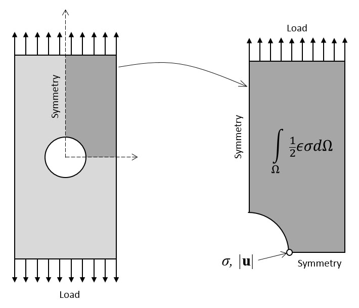 A schematic of a finite element model for a loaded plate with a hole.
A simple finite element model of a loaded plate with a hole. Symmetry is used to reduce the model size, and several different metrics can be defined to study mesh refinement.
A schematic of a finite element model for a loaded plate with a hole.
A simple finite element model of a loaded plate with a hole. Symmetry is used to reduce the model size, and several different metrics can be defined to study mesh refinement.
While choosing a metric, it is important to remember that different metrics will have different convergence behavior. This is illustrated in the figure below, showing different meshes being used to solve the same FEA model. These meshes differ in terms of the element size and are compared in terms of the number of degrees of freedom (DOF) within the model. The DOF is related to the number of nodes, the computational points that define the shape of each finite element. The computational resources required to solve an FEA model are directly related to the number of DOF.
From the figure below, it appears as if certain metrics converge faster than others, but it is important to keep in mind that the rate of mesh convergence for a particular problem statement is dependent upon which mesh refinement technique is used.
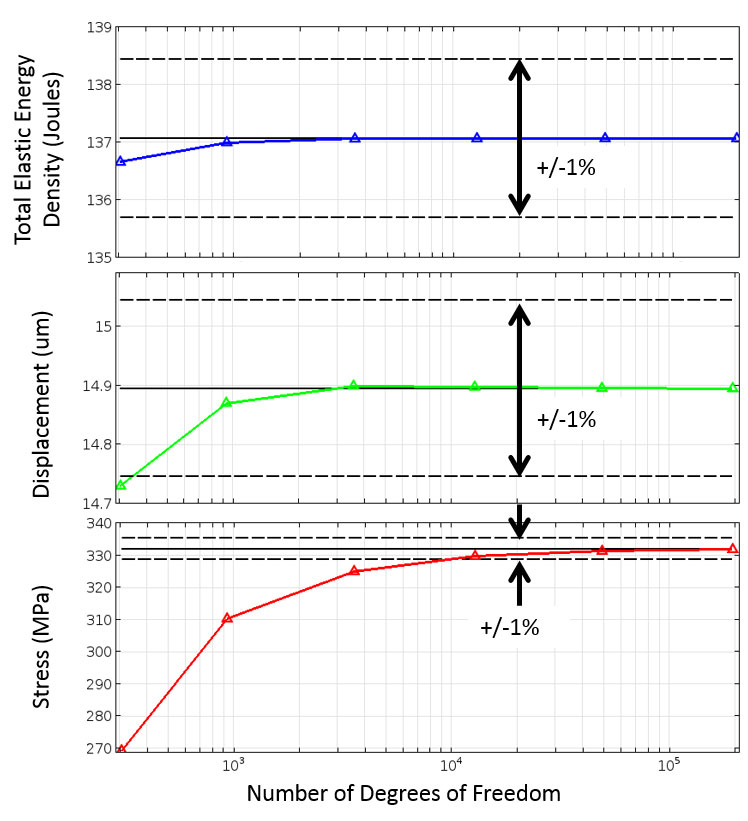 Plots illustrating the convergence of the finite element method under different metrics.
Convergence of a global metric (top), a local metric based upon the solution field (center), and a local metric based upon the gradient of the solution (bottom) with 1% error bars compared to the most refined solution. The same meshes were used for the three cases.
Plots illustrating the convergence of the finite element method under different metrics.
Convergence of a global metric (top), a local metric based upon the solution field (center), and a local metric based upon the gradient of the solution (bottom) with 1% error bars compared to the most refined solution. The same meshes were used for the three cases.
Different Mesh Refinement Techniques
When it comes to mesh refinement, there is a suite of techniques that are commonly used. An experienced user of FEA software should be familiar with each of these techniques and the tradeoffs between them.
Reducing the Element Size
Reducing the element size is the easiest mesh refinement strategy, with element sizes reduced throughout the modeling domains. This approach is attractive due to its simplicity, but the drawback is that there is no preferential mesh refinement in regions where a locally finer mesh may be needed.
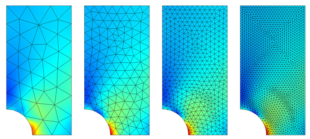 Reducing the element size as a mesh refinement strategy.
The stresses in a plate with a hole, solved with different element sizes.
Reducing the element size as a mesh refinement strategy.
The stresses in a plate with a hole, solved with different element sizes.
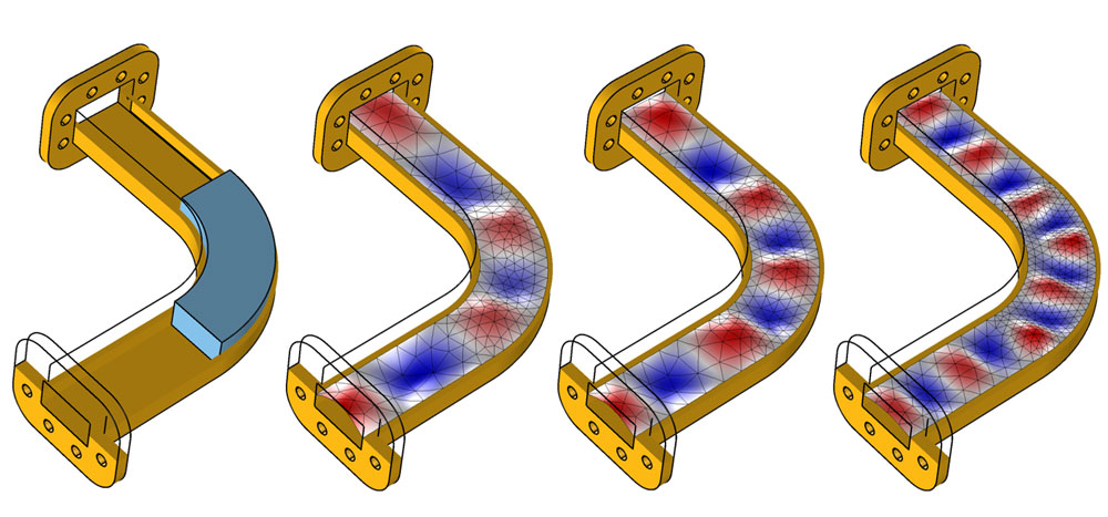
Increasing the Element Order
Increasing the element order is advantageous in the sense that no remeshing is needed; the same mesh can be used, but with different element orders. Remeshing can be time consuming for complex 3D geometries or the mesh may come from an external source and cannot be altered. The disadvantage to this technique is that the computational requirements increase faster than with other mesh refinement techniques.
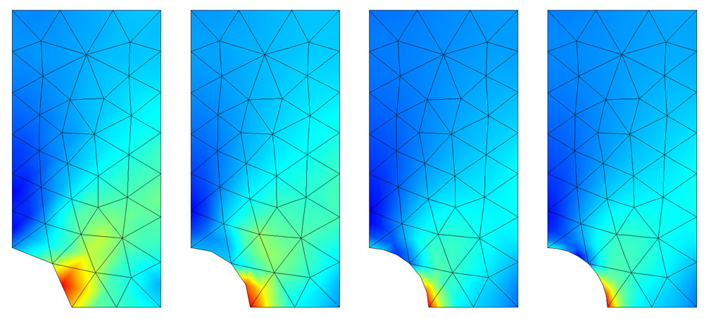 A series of simulations illustrating increases in the element order.
The same finite element mesh, but solved with different element orders.
A series of simulations illustrating increases in the element order.
The same finite element mesh, but solved with different element orders.
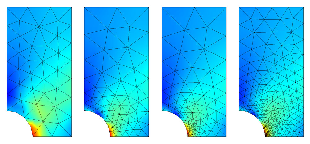
Global Adaptive Mesh Refinement
Global adaptive mesh refinement uses an error estimation strategy to determine the point in the modeling domain where the local error is largest. The FEA software then takes this error estimation and uses the information to generate an entirely new mesh. Smaller elements are used in regions where the local error is significant, and the local error throughout the model is considered. The advantage here is that the software will do all of the mesh refinement. The drawback is that the user has no control over the mesh. As such, excessive mesh refinement may occur in regions that are of less interest, regions where a larger local error is acceptable.
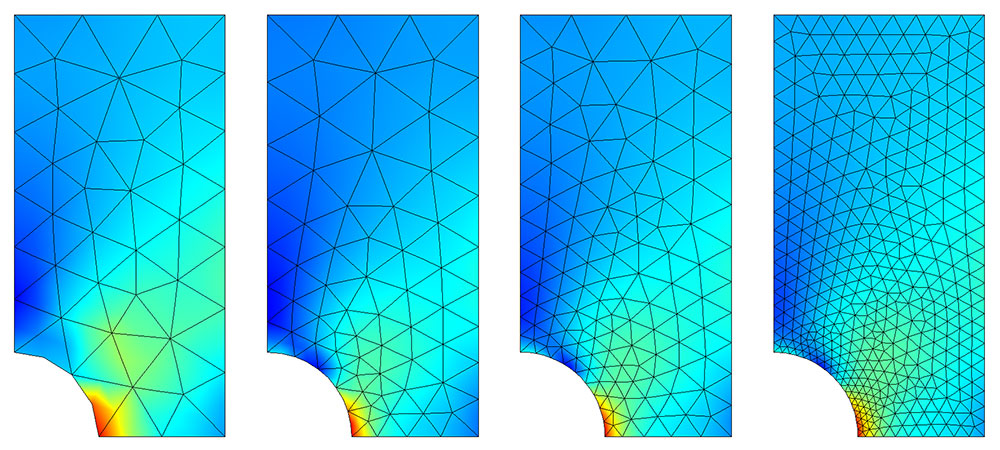 An example of using global adaptive mesh refinement.
Global adaptive mesh refinement changes the element sizes in a nonuniform manner.
An example of using global adaptive mesh refinement.
Global adaptive mesh refinement changes the element sizes in a nonuniform manner.
Local Adaptive Mesh Refinement
Local adaptive mesh refinement differs from global adaptive mesh refinement in that the error is evaluated only over some subset of the entire model space, with respect to a specific metric. For example, it is possible to refine the mesh such that stresses at the boundary of a hole are more accurately resolved. This meshing strategy will still remesh the entire model with the objective of reducing the error in one region. If a logical and desirable local metric exists with respect to which mesh can be refined, the local adaptive approach is superior to global adaptive mesh refinement.
 Simulations demonstrate the use of the local adaptive approach to refining meshes.
Local adaptive mesh refinement with respect to the stresses at a point.
Simulations demonstrate the use of the local adaptive approach to refining meshes.
Local adaptive mesh refinement with respect to the stresses at a point.
Manually Adjusting the Mesh
The most labor intensive approach is for the analyst to manually create a series of different finite element meshes based upon the physics of the particular problem and an intuition as to where finer elements may be needed. For 2D models, a combination of triangular and quadrilateral elements can be used. In the case of 3D models, a combination of tetrahedral, hexahedral (also called bricks), triangular prismatic, and pyramidal elements can be used. While triangular and tetrahedral elements can be utilized to mesh any geometry, the quadrilateral, hexahedral, prismatic, and pyramidal elements are helpful when the solution is known to vary gradually along one or more directions. By elongating, or shrinking, elements in certain directions, the mesh can be tuned to the variation in the fields.
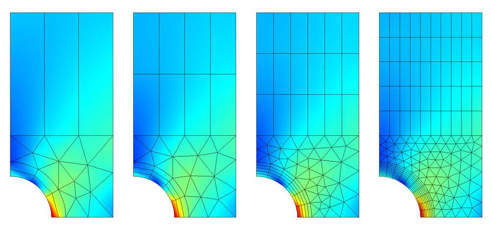 Manually created mesh of a plate featuring a hole.
A manually created mesh of a plate with a hole. Varying sizes of triangular and elongated quadrilateral elements are used.
Manually created mesh of a plate featuring a hole.
A manually created mesh of a plate with a hole. Varying sizes of triangular and elongated quadrilateral elements are used.
The manual meshing approach requires the most experience and a working understanding of the finite element method and the physics being solved. However, when done correctly, the savings on time and resources can be significant.
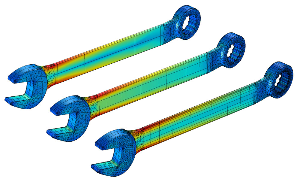 Manual mesh refinement of a wrench.
Manual mesh refinement of a wrench using different element types.
Manual mesh refinement of a wrench.
Manual mesh refinement of a wrench using different element types.
Time-Domain and Frequency-Domain Meshing
Along with all of the above techniques, additional considerations should be kept in mind when meshing problems that have time-varying loads. A model with nonlinear material responses or arbitrary time-varying excitations would need to be solved in the time domain. On the other hand, if the applied excitation is of a single frequency or a range of known frequencies and the material properties are linear, then it is preferred for the modeling to take place in the frequency domain. There are additional mesh refinement strategies for each of these cases.
Time-Adaptive Mesh Refinement
Time-adaptive mesh refinement remeshes the model at distinct time intervals and considers an error estimate of the solution at each interval as the metric by which to remesh the model. This is useful when the regions requiring good mesh resolution move over time.
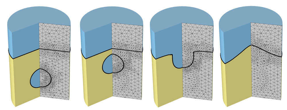 The time-adaptive mesh refinement of a rising bubble model.
Time-adaptive mesh refinement of a model of a rising bubble solved with a two-phase flow model. The finite element mesh is finer around the phase boundary.
The time-adaptive mesh refinement of a rising bubble model.
Time-adaptive mesh refinement of a model of a rising bubble solved with a two-phase flow model. The finite element mesh is finer around the phase boundary.
Wavelength-Adaptive Mesh Refinement
When modeling in the frequency domain, both the range of excitation frequencies and the material properties are known ahead of time. Thus, it is possible to predict the wavelength in all modeling domains. The element size must be sufficiently smaller than the wavelength, such that the element polynomial basis functions resolve the waves.
 A series of simulations illustrate the wavelength adaptive approach to refining mesh.
Microwave waveguide with a dielectric load (cutout view). Wavelength adaptive mesh refinement alters the element size based upon the frequency and material properties.
A series of simulations illustrate the wavelength adaptive approach to refining mesh.
Microwave waveguide with a dielectric load (cutout view). Wavelength adaptive mesh refinement alters the element size based upon the frequency and material properties.
Summary and Future Trends in Finite Element Meshing
The key point to keep in mind with all of these approaches is that, no matter which method is used, they will all converge toward the same solution for the posed problem. The difference between these various approaches is only in the rate at which they converge. This is, however, a significant practical difference. Depending upon the problem, one technique may converge much faster than others, and no one refinement strategy is appropriate in all circumstances. Every problem will have its unique meshing challenges, which continues to pose difficulties for analysts.
Some changes are underway that will ease these challenges. One of the most important developments over the last few years has been increasingly easy access to affordable cloud computing resources, enabling the running of several different cases in parallel. This allows analysts to study many model and mesh variations in much less time, giving them the ability to quickly address all of the uncertainties.
The algorithms used to generate the meshes themselves are also continuously improving and taking greater advantage of multicore computing. Additionally, the solvers are becoming more efficient, with the ability to solve huge models on cluster computers. All of these changes will provide more accurate solutions in less time, while accelerating the analysis and design process.
Published: January 6, 2016Last modified: February 21, 2017