Electroquasistatics, Theory
Time-Varying Current
For time-varying electric fields and currents, when magnetic effects are negligible, the steady currents equation can be generalized by combining the conservation of currents equation:
(1)

with Gauss's law:
(2)

which results in the following equation:
(3)

Assuming the field variations are sufficiently smooth, this equation can be reorganized into:
(4)

where the total current, which includes the displacement current, is:

Inserting the constitutive laws for linear materials:
(5)

and:
(6)

gives:
(7)

Inserting the equation for the electric potential:
(8)

then gives:
(9)

Note that by using the electric potential, it is implicitly assumed that there are no magnetic effects.
Time-Varying Current Equations and Boundary Conditions at Material Interfaces
The basic boundary conditions for electroquasistatics are summarized in the table below:
| Equation Name | Differential Form | Integral Form | Boundary Condition |
|---|---|---|---|
| Current conservation |  |
 |
 |
| Faraday's law (steady currents) |  |
 |
 |
where  is the total charge and
  is the current along the surface normal.
Time-Harmonic Fields
When fields are time varying and sinusoidal, the equations for electroquasistatics can be simplified by using phasors, which are field quantities that encode both amplitude and phase information by using complex-valued expressions. As a background to using phasors, consider the Fourier expansion of the time evolution of a field quantity; for example, the electric potential:
(10)

where higher-order terms include the overtones proportional to  ,
,  , etc.
For a sinusoidal field, the overtones vanish and only the zeroth- (constant-) and first-order Fourier terms remain.
Time-Harmonic Electric Currents
If the zeroth-order term is substituted into the electroquasistatic equation for linear materials, then due to the time invariance of  , the result is the conservation of the steady currents equation. Also, due to the linearity of the material and the equation, the zeroth-order and first-order parts can be treated independently. Therefore, the interesting remaining equation comes from the harmonic (first-order) term:
(11)

By letting the time derivative operate on just the time-varying parts and using the fact that the exponential function is always nonzero, this can be simplified to:
(12)

Here, it is implicitly assumed that the material properties are time invariant. Furthermore, the subscript 1 is dropped from the electric potential field to simplify the notation. This equation is the time-harmonic version of the electroquasistatic equation. The electric potential in this equation is a phasor quantity and may have a nonzero phase shift and therefore be complex valued:
(13)

The quantity:
(14)

can be interpreted as a complex-valued conductivity.
This version of the electroquasistatic equation is a time-harmonic generalization of the steady currents equation:
(15)

where:
(16)

is the time-harmonic current density.
This can also be written as:

with the individual contributions from the conductive current density and the displacement current density. At material interfaces, the continuity condition for the current is:

In the important case where there is no normal current on the external surface, and where  , this condition becomes:

In other words, the continuity condition at material interfaces is the same as for the electrostatics case.
Time-Harmonic Electrostatics
Dividing the electroquasistatic equation by  gives another version of the equation:
(17)

where the quantity:
(18)

can be interpreted as a complex-valued permittivity.
This version of the electroquasistatic equation is a time-harmonic generalization of the electrostatics equation:
(19)

where:
(20)

is the time-harmonic displacement field.
Summary of Time-Harmonic Formulations
The following table lists the two equations for time-harmonic electroquasistatics together with the associated material property and constitutive relationship:
| Equation Name | Equation | Material Property | Constitutive Relationship |
|---|---|---|---|
| Time-harmonic current density (time-harmonic electric currents) |
|
|
 |
| Time-harmonic displacement field (time-harmonic electrostatics) |
|
|
 |
It can be noted that, in the limit where the frequency goes to zero, the first equation remains well defined and becomes the equation of steady currents. On the other hand, in this limit, the imaginary part of the complex permittivity becomes unbounded for the second equation. However, if the material is a perfect insulator and the electric conductivity is zero, the second equation becomes independent of frequency and identical to that of electrostatics.
This indicates that, for the static case, the conservation of the current equation is useful for modeling perfect conductors ( ), and the electrostatics equation is useful for modeling perfect insulators (
 ). For good conductors and low-enough frequencies, the imaginary part of the time-harmonic current density equation can be neglected as long as
  . Likewise, for good insulators, the imaginary part of the time-harmonic displacement field equation can sometimes be neglected, but for certain materials at higher frequencies, the loss (
 ) becomes frequency dependent and the imaginary part becomes important.
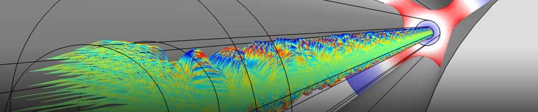
The ion trajectories in a quadrupole mass spectrometer.
This type of spectrometer sorts particles by using a clever combination of a static and time-harmonic electric potential,  . By tuning the harmonic frequency (here, at 4 MHz) and the strengths of the static and harmonic fields, only particles of a certain mass are transmitted through the device.
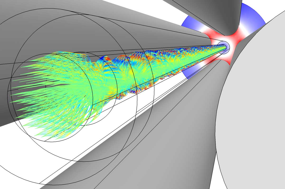
The ion trajectories in a quadrupole mass spectrometer.
This type of spectrometer sorts particles by using a clever combination of a static and time-harmonic electric potential, . By tuning the harmonic frequency (here, at 4 MHz) and the strengths of the static and harmonic fields, only particles of a certain mass are transmitted through the device.
Last modified: February 13, 2019