
Analysis of Deformation
Analysis of Deformation in Solid Mechanics
The analysis of deformation is fundamental to the study of all solid mechanics problems.
Solid mechanics equations are usually formulated by tracking a certain volume of material as it translates, rotates, and deforms. This is called a Lagrangian formulation, as opposed to the Eulerian formulation commonly adopted in many other fields of physics, such as fluid flow analysis. The basis of an Eulerian formulation revolves around the flux in and out of a control volume that is fixed in space.
In the context of finite element analysis, two different variants of Lagrangian formulations are commonly used:
In the total Lagrangian formulation, the equations are based on the original configuration of the body
In the updated Lagrangian formulation, the equations are based on the current configuration of the body
These two formulations are mathematically equivalent in the sense that one can be transformed into the other by a formal application of a number of transformations. However, the formulations have different merits when it comes to the numerical efficiency of the finite element formulations.
The development of the theory assumes that the solid material can be treated as a continuum. The length scale is significantly larger than the molecular scale so that properties are homogeneous, but small enough to be considered as infinitesimal from the mathematical point of view.
Coordinate Systems and Displacements
Let the coordinates  denote the original location of a material particle. We can consider as a label that sticks to a certain particle throughout the deformation history. This coordinate system is called the material coordinate system (or material frame).
At a certain time  , the particle has moved to a new location,
  . For simplicity, let us assume that both sets of coordinates have the same origin and orientation. The coordinates
  are in the spatial coordinate system (or spatial frame). The spatial coordinate system is fixed in space, whereas the material coordinate system is fixed to the body.
The vector pointing from the original location of a point in the body to its new location is the displacement vector,  . Since the original coordinates are the independent variables, this is a Lagrangian formulation. Thus, the displacement provides the transformation from the material to the spatial frame,
  .
.
 Relation between the material and spatial coordinates of a point.
Relation between the material and spatial coordinates of a point.
Relation between the material and spatial coordinates of a point.
As long as the displacement field does not represent a pure rigid body motion, there are local changes in the shape of the material, which are called strains or stretches. These changes may consist of a change in volume or shape of a local small domain. The strains will cause internal forces in the material (stresses) and possibly even failure. In order to successfully describe the material behavior, the distortion must be described in a way that is independent of, for example, rigid body motions. There are several ways in which we can describe the straining of the material, as we will discuss below.
The Deformation Gradient
The deformation gradient  is defined as

where  is the identity tensor. In matrix form

The deformation gradient contains the full information about the local rotation and deformation of the material. It also shows, for example, how a small line segment in the undeformed body,  , is rotated and stretched into a line segment in the deformed body,
  , since
  . The first column in the tensor (when viewed as a matrix) gives the scale and orientation of a line segment originally oriented in the X-direction and so on. Mathematically speaking, is the Jacobian matrix of the transformation from to , so its determinant,
  , is the local volume scale factor. For an incompressible material,
  .
.
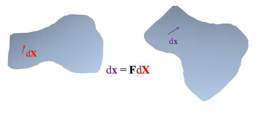 An infinitesimal line segment is stretched and rotated by the deformation gradient.
An infinitesimal line segment is stretched and rotated by the deformation gradient.
An infinitesimal line segment is stretched and rotated by the deformation gradient.
By making use of the Polar decomposition theorem, which states that any second-order tensor can be decomposed into a product of a pure rotation and symmetric tensor, it is possible to separate the rigid body rotation from the deformation:

This can be interpreted as a deformation described by the right stretch tensor  , followed by a rigid rotation by the pure rotation matrix
  . Thus, if there is no rotation, the right stretch tensor is the deformation gradient, so the interpretation of is similar to that of .
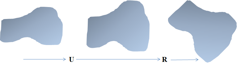 Decomposition into deformation followed by a rotation.
Decomposition into deformation followed by a rotation.
Decomposition into deformation followed by a rotation.
It is equally possible to decompose the deformation gradient into

The rigid body rotation is performed first and the rotated volume is then deformed. The deformation is described by the left stretch tensor  .
.
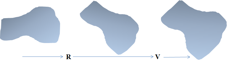 Decomposition into a rotation followed by deformation.
Decomposition into a rotation followed by deformation.
Decomposition into a rotation followed by deformation.
The two stretch tensors are related through a pure rotation; for example,  . Here, the fact that the transpose of a rotation matrix is also its inverse (
 ) is used.
Computing the polar decomposition in practice is computationally expensive, so it is mostly avoided. However, this concept is very useful in theoretical considerations.
It is possible to compute a measure of the deformation, which is independent of the rotation, without actually knowing the rotation matrix:

The  tensor is called the right Cauchy-Green deformation tensor.
This tensor is often used when describing the constitutive properties of hyperelastic materials, for example. Since it is formed only from the tensor, it describes the deformation of the material "before" rotation.
Similarly,

The  tensor is called the left Cauchy-Green deformation tensor.
Both and are independent of the rotation, but they describe the deformation in two different coordinate systems. The tensor is a material tensor, describing the deformation in the material coordinate system, while is a spatial tensor, describing the deformation in the spatial coordinate system.
Stretch
Stretch is, in an informal sense, defined as the ratio between current length and original length,

so that the stretch in the undeformed state is 1.
In a more general setting, the eigenvalues of the and tensors are of special interest. The three eigenvalues of ( ,
,  , and
, and  ) are called principal stretches. Their corresponding eigenvectors give three orthogonal directions (in the material coordinate system). If a small cube with edges along these directions is studied, it will be deformed into a cuboid but maintain the right angles between all of the edges. The changes in edge lengths are given by the principal stretches.
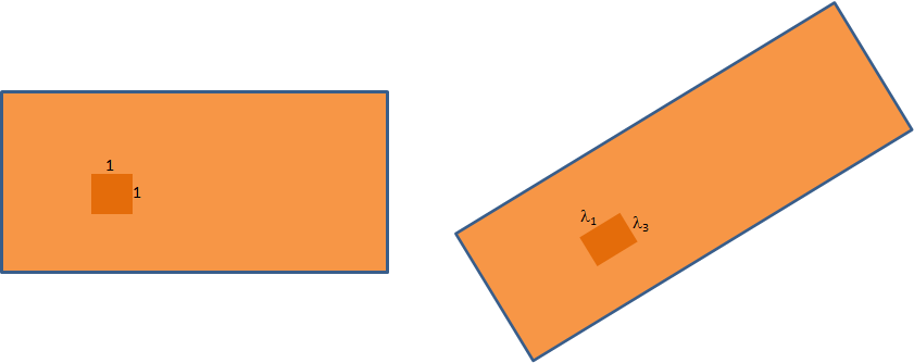 Principal stretches (assuming that the thickness does not change so that λ2 = 1).
Principal stretches (assuming that the thickness does not change so that λ2 = 1).
Principal stretches (assuming that the thickness does not change so that λ2 = 1).
The change in volume can thus be written as the product of the principal stretches:

The computationally more convenient tensor has the same principal directions as , but the eigenvalues are  ,
,  , and
, and  . Principal stretches are thus usually computed using rather than .
For an undeformed material (rigid body motion only),  . This fact gives a clue to why , in practice, is mostly used for describing materials with large stretches like rubber. For materials like metals, the strains are often of the order of
  to
to  . If stretches were to be used as a measure of the material strain, a stretch range of 0.99 to 1.01, or maybe even 0.9999 to 1.0001, would be used to describe the deformation.
The left Cauchy-Green deformation tensor also has the principal stretches as eigenvalues. The principal directions, however, are oriented with respect to the spatial directions, since describes the stretches after the rigid body rotation.
Strain Tensors
To get a deformation measure that is based at zero, the identity tensor is subtracted from . This gives the Green-Lagrange strain tensor  , defined as

This tensor also describes the deformation of the material prior to any rotation, but with all components as zero in the undeformed state. On component form, it can be written as

where summation over repeated indices (Einstein's summation convention) is assumed.
An example of a diagonal element of the Green-Lagrange strain tensor is

and an example of an off-diagonal element is

The eigenvalues of the Green-Lagrange strain tensor are called principal strains and have the same (material frame) orientations as the principal stretches.
When both strains and rigid body rotations are small, the quadratic terms in the Green-Lagrange strain tensor can be ignored. This leads to the well-known engineering strain tensor,

having components such as

and

The diagonal terms of the strain tensor are called normal strains or direct strains. They describe the extension along each of the coordinate axes. The off-diagonal terms are the shear components of the strain tensor and describe changes in the angles between line segments. There is a risk of confusion in the terminology here, since in engineering, it is customary to assign the name "shear strain" to the quantity  . This is because
  directly measures the change of angles (in radians).
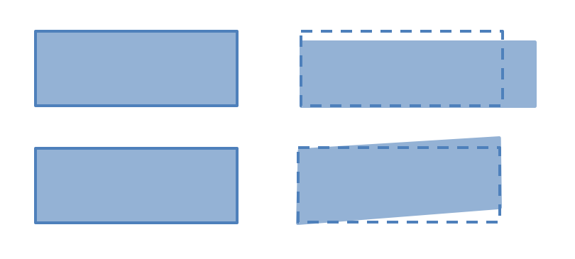 Normal strain (top) and shear strain (bottom)
Normal strain (top) and shear strain (bottom)
Normal strain (top) and shear strain (bottom)
The shear strains give an isochoric deformation; that is, a deformation without volume change. The relative volume change is, for small strains, given by the sum of the direct strains:

Changing the Perspective
If we take the deformed shape as the starting point of the analysis, it is possible to perform a similar development of the theory. This will not be covered in detail here, but the steps are analogous. The original location and displacements are viewed as a function of the current location,  , so all derivatives are taken with respect to the spatial coordinates. A line segment with the current length has its origin in the line segment , which can be found using
  .
.
The Almansi strain tensor is defined as

When writing out the components,

Note that the derivatives are now taken with respect to the spatial coordinates.
True Strain
Sometimes the term true strain is used. In a uniaxial definition of true strain, the strain increment is defined as

The definition of true strain is based on the current length, so that after integration,

which is why the true strain is also called logarithmic strain. The generalization to 3D is called the Hencky strain tensor,

A Comparison of Strain Measures
If a bar with initial length  is extended (or compressed) a distance
  , then the different strain measures for the strain in the axial direction are as follows.
Engineering strain:

Stretch:

Green-Lagrange strain:

Almansi strain:

True strain:

In the graph below, we can see that all strain measures coincide well up to approximately ±10%, but at higher strains, there are significant differences. The engineering strain and stretch are both proportional to the deformation and only differ by a vertical shift.
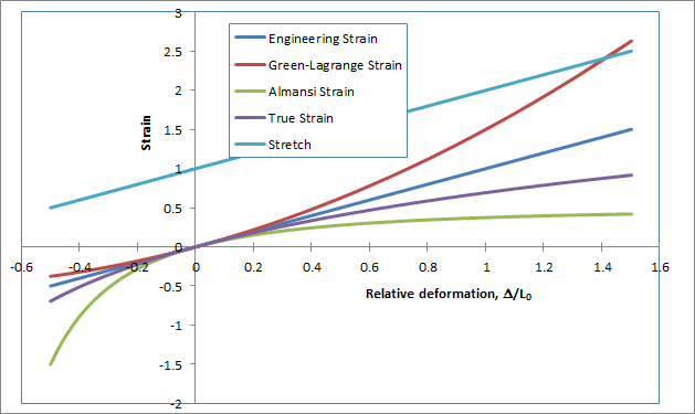 Comparison between different strain measures.
Comparison between different strain measures.
Comparison between different strain measures.
Compatibility of Strains
Since a strain tensor consists of derivatives of the displacements, not all strain fields are admissible. There are only three components of the displacement vector, so integration of various strain components cannot give a unique set of displacements unless they fulfill certain compatibility criteria. For the engineering strains, the following equations must be fulfilled:

Due to the symmetry of the strain tensor, only 6 out of these 81 equations are nontrivial. These are

Velocity Gradient and Time Derivatives of Strain
Related to the deformation gradient is also the velocity gradient. It is defined as the spatial gradient of the velocity vector,

The velocity gradient can be decomposed into symmetric and antisymmetric parts, called the strain rate tensor and spin tensor, respectively:

The velocity gradient has an important relation to the time derivative of the deformation gradient:

Using this result, the time derivative of the Green-Lagrange strain can also be expressed in the velocity gradient,

The last identity is due to the symmetry of the strain tensor.
Deformation Analysis Example: Rigid Body Rotation
Consider a rigid body rotation by an angle  in the xy-plane:
If the origin of the coordinate system is assumed to be at the lower left corner, the new location of a certain point (x, y) can be written as a function of the original coordinates (X, Y) as

The displacements are then

The deformation gradient can then be computed from its definition, giving

so that the right Cauchy-Green tensor is

In the same way, the left Cauchy-Green tensor is  . From definitions, it is clear that the Green-Lagrange and Almansi strain tensors are identically zero. Also, since all principal stretches have the value one, the Hencky strain tensor is zero.
The engineering strain tensor, however, contains the following values

For small angles, a series expansion gives

At first glance, this looks like a small error. However, strains are already significant at small numerical values. In a metal, substantial stresses typically occur at strains of the order of 0.01%. This means that using the engineering strain tensor will cause significant errors, even at a 1° rigid body rotation.
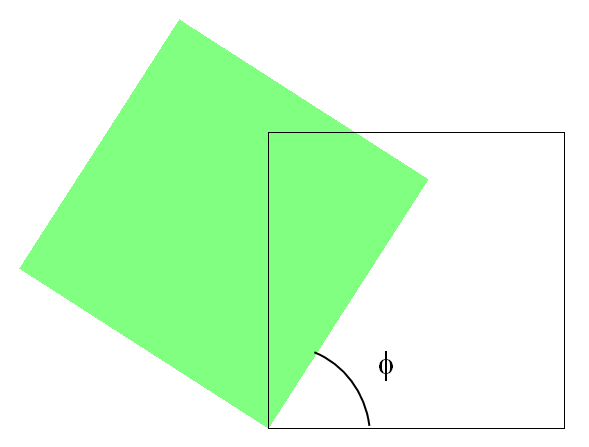
Deformation Analysis Example: Large Shearing
A square is sheared by an angle  into a rhombus, as shown in the figure below. There is no out-of-plane deformation.
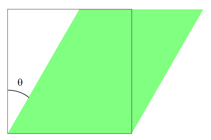
Simple shear.
Simple shear.
The mapping from the material to the spatial frame is (Z is the out-of-plane direction):

The expression  is the amount of shear, which gives the following displacement fields

The deformation gradient will then be

We immediately see that  , so that the deformation is volume preserving. This matches the expectations from the above figure as well, since the original square has been deformed into a rhombus of the same area.
The right Cauchy-Green stretch tensor and Green-Lagrange strain tensor are

and

respectively.
The diagonal elements of the Green-Lagrange strain tensor can be interpreted. A fiber originally oriented along the X-axis has not been extended, whereas a fiber along the Y-axis has been stretched. The new length of this fiber, however, cannot be directly extracted from the strain tensor.
For small angles,  and
and  , the engineering strain tensor for pure shear is retrieved:

The polar decomposition of  can, with some effort, be computed. Setting
  , then

and

where  .
.
The principal stretches, which are the eigenvalues of , are commonly sorted in descending order. They are

The second principal stretch  , since there is no out-of-plane stretching.
The eigenvectors of the right stretch tensor are the principal stretch axes. In this example, they can be expressed as
 ,
,  , and
, and 
To further investigate the problem numerically, the shear angle is set to  . Then,
  ,
,  , and
, and  . The deformation gradient becomes

The rigid part of the rotation, , can be found numerically from the rotation matrix, since  .
.
The principal stretches are

The orientation of the first principal stretch axis is 58.3° from the horizontal axis.
In the figure below, the deformation is decomposed into a pure stretch and pure rotation. The blue square is oriented so that it matches the principal stretch directions; it is rotated 58.3°. We can see that it assumes a pure rectangular shape and that the orientation does not change during the stretching part of the decomposed displacement.
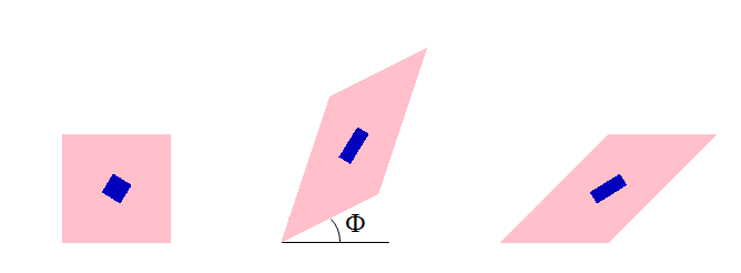 Original configuration (left), stretching only (middle), and stretching followed by rotation (right).
Original configuration (left), stretching only (middle), and stretching followed by rotation (right).
Original configuration (left), stretching only (middle), and stretching followed by rotation (right).
Last modified: March 11, 2021