Acoustic-Structure Interaction
Acoustic-Structure Interaction Creates Sound
Acoustics is the physics of sound – the sensation of very small and rapid changes in the acoustic pressure above and below the atmospheric pressure. We describe these changes as pressure waves propagating in space and time. The wave crests and troughs represent the pressure maxima and minima, respectively.
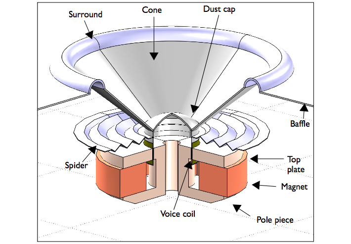
When a vibrating structural object disturbs the gas or liquid (the fluid) carrying the acoustic pressure waves, sound is created. The vibrating object in question may be a plate, membrane, or solid. This process is also referred to as acoustic-structure interaction. The pressure waves in the fluid medium also produce vibrations in the solid. The interaction is two-way, although sometimes, the interaction in one direction is dominating. An everyday example of this is the speaker cone in a sound system.
Acoustic-structure interaction involves the coupling of physics from two different fields: acoustics and structural mechanics. In some applications, both the acoustic pressure waves in the fluid and the vibrations of the solid are strong enough to affect each other significantly, resulting in two-way coupling.
An Example of Acoustic-Structure Interaction
In a loudspeaker, the structural displacements of the voice coil impose a vibration of the speaker cone membrane. This leads to pressure changes in the surrounding air and creates the sound signal heard by the listener.
If you observe a bass speaker cone as it produces sound at a very low frequency, you may notice that it moves back and forth. When it moves forward, the cone compresses the air in front of it, thereby increasing the air pressure. As it then moves back, beyond its initial position, it reduces the air pressure. The continued movement of the cone causes a wave to radiate at alternating high and low pressure at the speed of sound. The air surrounding the speaker cone also influences the cone movements, for example, in terms of so-called added mass. These effects need to be taken into account when designing and optimizing speakers.
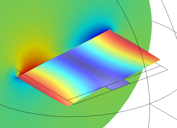
Deformation and velocity fluctuations of a vibrating micromirror.
Deformation and velocity fluctuations of a vibrating micromirror.
In other cases, acoustic pressure waves in the medium are used to produce vibrations in a solid, such as in ultrasound imaging or in nondestructive impedance testing.
Viscous and Thermal Damping of Vibrations
Thermal and Viscous Losses
Thermal and viscous losses come into play when sound propagates in small structures, such as small transducers and receivers. This causes the sound waves to weaken, or attenuate, but most importantly, the structural vibrations are damped. These effects are typically observed in response measurements where resonances are damped (rounded with high Q-values) and shifted down in frequency. Including these effects is essential when, for example, modeling miniature transducers like MEMS microphones. The study of these loss mechanisms falls under thermoacoustics, a subset of the acoustics field. Viscosity and thermal conduction effects typically lead to significant losses (energy dissipation) near the walls of the structure in the acoustic boundary layer.
Bulk thermal conduction and viscosity can also lead to losses when acoustic signals (sonar signals, for instance) are transmitted over long distances and are weakened. In air, it is important to consider bulk losses only at very high frequencies, but they can be disregarded at audio frequencies.
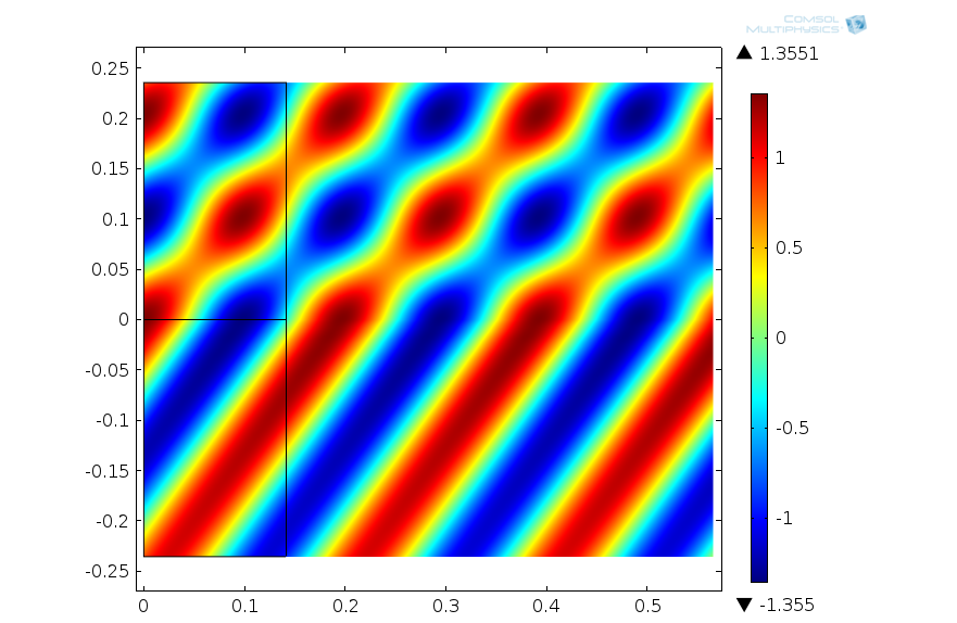
Acoustic pressure for an oblique incident pressure wave on a porous sediment layer.
Acoustic pressure for an oblique incident pressure wave on a porous sediment layer.
The Couplings
In classic acoustics, when solving the Helmholtz equation or the scalar wave equation, the physical assumption is that the fluid is inviscid and isentropic. In this case, slip conditions exist on solid walls and coupling is done normal to the surface. Hence, the acoustic-solid coupling is a multiphysics phenomenon, where the acoustic pressure causes a load on the solid and the structural acceleration is exciting the fluid (the normal acceleration of the solid wall).
When the fluid is modeled including the viscous and thermal losses, both a mechanical and thermal condition must be specified at the solid surface. The no-slip condition must apply, ensuring continuity in the velocity; the movement of the solid is equal to the movement of the fluid. Finally, the acoustic fluctuations in the temperature are typically assumed to be isothermal at walls (thermal conduction is much larger in solids than in fluids). These conditions lead to a tightly coupled multiphysics problem. For harmonic perturbations, it can be thought of as fluid-structure interaction (FSI) in the frequency domain.
Porous Materials
Another area where pressure waves and structural vibrations are closely linked is when sound propagates in porous materials. The pressure fluctuations in the saturating fluid interact with different elastic waves (shear and longitudinal) in the porous material. Because the pores are often small in size, losses exist here that introduce damping in the system. Moreover, the porous domain can be coupled to pure solid structures or to pure fluid domains, introducing a multitude of multiphysics couplings.
There are several ways of describing the propagation of waves in porous materials. One of the most detailed involves solving Biots equations. They account for the coupled propagation of elastic waves in the elastic porous matrix and pressure waves in the saturating pore fluid. This includes the damping effect of the pore fluid. Another approach is to treat the porous matrix and saturating pore fluid as a homogenized equivalent fluid. In this case, only the pressure waves are modeled including descriptive losses. The loss models can range from pure empirical models based on measurements to analytical or semianalytical phenomenological models; examples include the Delany-Bazley-Miki or the Johnson-Champoux-Allard models.
Published: November 6, 2014Last modified: February 21, 2017