

When performing structural mechanics analyses, you will inevitably encounter the concept of geometric nonlinearity. In this blog post, we discuss what is meant by geometric nonlinearity and when you should take this effect into consideration.
An Introduction to Geometric Nonlinearity
Geometric nonlinearity may not even be explicitly introduced in a fundamental course on structural mechanics. In fact, geometric linearity is often tacitly assumed. In a geometrically linear setting, the equations of equilibrium are formulated in the undeformed state and are not updated with the deformation. This may sound a bit alarming at first, since computing deformations is what structural mechanics is all about.
However, in most engineering problems, the deformations are so small that the deviation from the original geometry is not perceptible. The small error introduced by ignoring the deformations does not warrant the added mathematical complexity generated by a more sophisticated theory. This is why a vast majority of analyses are made with an assumption of geometric linearity.
There are a number of cases where the deformation cannot be ignored, and not all of these cases comprise deformations that you would intuitively think of as being large.
Effects of Including Geometric Nonlinearity
The most important effects on the mathematics when you include geometric nonlinearity in COMSOL Multiphysics are:
- A distinction is made between the Spatial and the Material frame. The spatial coordinates of a certain point (\mathbf x) differ from the material coordinates of the same point (\mathbf X) by the the displacement vector (\mathbf u), so that \mathbf x = \mathbf X + \mathbf u. It will thus matter whether you use uppercase or lowercase coordinate names in expressions.
- The strains are represented by the Green-Lagrange strain tensor instead of the engineering strains.
- The stresses are represented by the Second Piola-Kirchoff stress tensor.
- Pressure loads take the deformation into account. Normals to boundaries are updated and area changes caused by stretching are taken into account.
You can read more about different stress and strain tensors in this previous blog post, but a small digression into the strain measures is needed. To this end, let us look at the difference between linear and the full nonlinear strain by considering some components of the strain tensor.
The X-direction Green-Lagrange normal strain can be written as
If the quadratic terms are omitted, the familiar engineering strain is retrieved:
Similarly, for a shear strain, the Green-Lagrange strain component is
Again, the engineering strain is obtained by ignoring the nonlinear terms:
Large — or Not so Large — Rotations
When a structure rotates significantly, the engineering strains used in basic theory will no longer give a useful representation. Rigid body rotations will cause nonzero components of the engineering strain tensor. This will, through the constitutive law, cause stresses that for physical reasons should not appear in a rigid body. Another way of viewing this is that any useful strain tensor must be able to reflect the fact that there is no stretching or change of relative angles in a rigid body motion.
Consider a 2D body rotating rigidly in the xy-plane around the origin. A simple linear plane stress model in which a rectangular steel plate is rotated 10° is shown below.
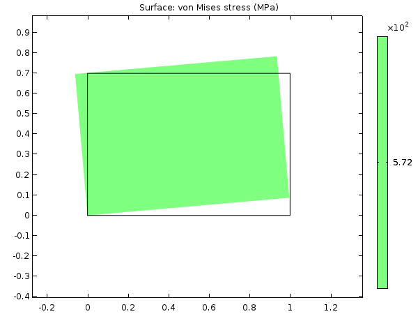
Equivalent stress in a rectangular steel plate at a 10° rotation with no geometric nonlinearity.
The result is an equivalent stress of 572 MPa, which is above the yield limit for the most common steel qualities. To see why this happened, let’s study the analytical solution:
A point originally placed at (X,Y) will then have moved to a new location (x,y), given by
x = X \cos(\phi)-Y \sin(\phi) \\
y = X \sin(\phi) + Y \cos(\phi)
\end{matrix}
This means that the displacements (u,v) are
u = x-X = X (\cos(\phi)-1)-Y \sin(\phi) \\
v = y-Y = X \sin(\phi) + Y (\cos(\phi)-1)
\end{matrix}
The engineering strains will then be
\epsilon_X = \frac{\partial u}{\partial X} = \cos(\phi)-1 \\
\epsilon_Y = \frac{\partial v}{\partial Y} = \cos(\phi)-1 \\
\epsilon_{XY} = \frac{1}{2}(\frac{\partial u}{\partial Y}+\frac{\partial v}{\partial X}) = -\sin(\phi)+ \sin(\phi) = 0
\end{array}
For a rigid body rotation, all strains should be zero, but clearly two of these strain components are not. A metal will often yield at a strain that is of the order of 0.001. A fictitious strain of this size will already occur at a rotation of 2.5°. To keep the strain lower than 0.0001, there must not be rigid rotations larger than 0.8°. This means that even at angles where you often would expect a “small angle approximation” to be sufficient, the geometrically nonlinear approach must be used.
Using the same rigid body rotation as above, but using Green-Lagrange strains instead, gives
Now this strain tensor component is zero for any value of the rotation. This property can be shown for the whole Green-Lagrange strain tensor and also for arbitrary rotations.
By using a geometrically nonlinear formulation, you can avoid having these kinds of stress artifacts. This is confirmed by solving the same problem with geometric nonlinearity enabled. The stress levels are now pure numerical noise; 12 orders of magnitude lower than the yield limit.
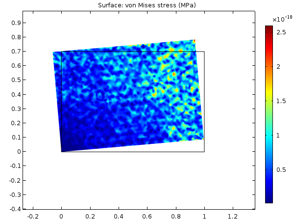
Equivalent stress at a 10° rotation while using geometric nonlinearity.
Stretching of Thin Structures
Consider the two beams in the sketch below:
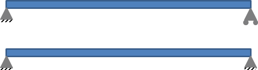
Beams with different end conditions.
At the right end, the upper beam is free to translate horizontally, while the lower beam is not. In a linear theory, these two end conditions are equivalent if the beam is subjected to a vertical load. There is no coupling between axial and bending action. However, in a geometrically nonlinear analysis, the different end conditions will lead to quite different results:
- When the end is free to move axially, the vertical displacement of the beam is almost the same as in the geometrically linear case.
- When the axial displacement is constrained, the vertical displacement will be smaller than in the linear case and have a strong nonlinear dependence on the load.
As the beam deflects, its center line will be stretched if the end cannot move inwards. This will introduce a significant axial force that will make the beam act similar to a wire in tension — the higher the tensile force, the more it will resist a transverse force.
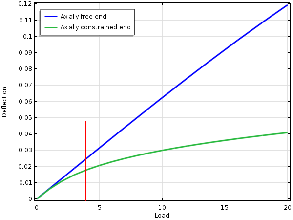
Midpoint deflection of a beam with a square cross section of 0.05 x 0.05. The red line indicates the load where the deflection in the linear analysis is 0.025 (half the height of the beam).
The same ideas also apply to plates and shells. If the boundary conditions are such that deflection will cause in-plane tension, then the plate will become significantly stiffer with increasing deflection.
There is a rule of thumb saying that if the deflection of the beam or plate in a linear analysis exceeds half of its thickness, then geometrically nonlinear effects should be considered. This is indicated by the red line in the figure above.
Stress Stiffening
As seen in the previous example, the stiffness of a structure can sometimes change significantly due to geometrically nonlinear effects. This is sometimes referred to as stress stiffening. The term is somewhat misleading, since it is also possible that the stiffness could decrease. If we were to add a compressive axial load to the beam above, its transverse stiffness would actually decrease.
Stress stiffening is important in, for example, rotating systems where the centrifugal forces can introduce significant tensile stresses. This causes the eigenfrequencies of the system to increase with the RPM.
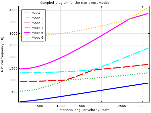
Campbell diagram showing how the natural frequencies of a rotating blade change with speed of rotation.
Often, the loads that cause the prestress are not the same as the one for which you actually perform the analysis. So there may be two distinct load systems that must be analyzed separately.
In COMSOL Multiphysics, there are two predefined study types specifically intended for the analysis of prestressed systems:
- Prestressed Analysis, Eigenfrequency
- Prestressed Analysis, Frequency Domain
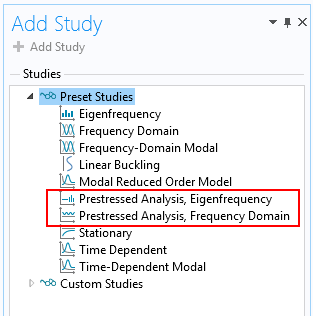
Study types intended for the analysis of prestressed structures.
These study types consist of two study steps in which step one is used for computing the prestress state. That study can be linear or nonlinear. The second study step is linear in itself, but includes the nonlinear terms caused by the geometric nonlinearity when setting up the stiffness matrix.
If you are interested in examples in which stress stiffening is important, please check out:
Buckling
Buckling, or the loss of stability when the load reaches a certain critical value, is caused by geometrically nonlinear effects. In COMSOL Multiphysics, there is a specific study type called Linear Buckling for computing the first order approximation to the critical load.
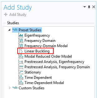
The Linear Buckling study type.
In the linear buckling study, an approximate buckling load is obtained by solving an eigenvalue problem.
As an alternative, you can trace the full nonlinear response up to the point of collapse, and even past it. In this case, you must increase the load in smaller steps. This approach is significantly more computationally expensive, but more accurate.
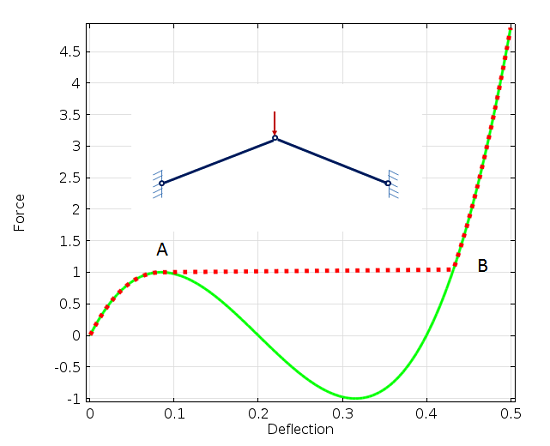
Load-deflection history with a buckling collapse at point A.
You can read more about buckling in this previous blog post.
Using Geometric Nonlinearity in COMSOL Multiphysics
Enabling Geometric Nonlinearity
Geometric nonlinearity is a property of the Study step. For those study types for which it is relevant, a check box is available in the settings for the study.
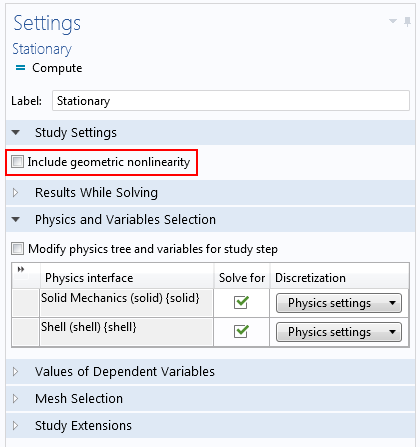
Settings for a stationary study.
Sometimes this check box is preselected and you cannot change it. This happens when you include certain physics nodes in the model tree that cannot be used in a linear context, such as:
- Hyperelastic material
- Large strain plasticity
- Contact
Note that most nonlinear material models, such as nonlinear elasticity or creep, do not assume geometric nonlinearity.
Solving a Problem with Geometric Nonlinearity
Geometrically nonlinear problems are often strongly nonlinear, and you need to consider that when supplying settings for the solver.
Think of the beam with the fixed end mentioned above. When solving the nonlinear problem, the solution after the first iteration will be the same as the solution to the linear problem so that all points on the beam move only vertically under a transverse load.
After the first iteration, there will thus be a significant axial elongation of the beam. Such an elongation is related to an axial force. As there is no net axial force (there is no external load in that direction), this force will end up as a residual for the next iteration. This unbalanced force may be larger than the applied load. To the nonlinear solver, this looks like a very nasty problem and the solver will often introduce damping.
Fortunately, these problems are often more well behaved than the numerics would indicate. You can then speed up the solution significantly by using a more aggressive iteration scheme than the default.
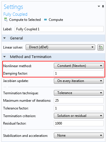
Settings for the Fully Coupled solver.
Using the Constant Newton scheme instead of the automatic adaptive scheme will cause the solver to make larger updates. The damping factor can be set to 1 (no damping) or possibly 0.9.
A problem where geometrical nonlinearity is the only source of nonlinearity will, in most cases, possess a unique solution for a certain load level. In this sense, it is possible to analyze the problem using a stationary analysis with a single load only. For convergence reasons, it is sometimes better to gradually increase the load using the parametric continuation solver.
An example of how the solver can be set up for a severely nonlinear problem is shown in our Pinched Hemispherical Shell tutorial model.
Final Remarks
As we have shown above, there are several cases in which geometric nonlinearities must be considered when solving structural mechanics problems. So why don’t we always include this effect in our models to be on the safe side?
- Even if the nonlinear effect is very small, invoking the nonlinear solver will give you a significantly longer solution time. This is not an issue for small models, but when you are working with several million degrees of freedom, a reduction of the solution time by a factor of two really matters.
- Sometimes you want to be able to compare to an analytical solution, and such solutions are often based on linear theory.
- You may need to follow a standard or analysis procedure where it is assumed that a linear approach is used.
- In a geometrically nonlinear problem, it is necessary to use the actual load. If you just want to do a conceptual study of a structural response, the solution may not converge if the estimated load was too large.


Comments (4)
Ivar Kjelberg
September 17, 2015Hi Henrik
Thanks again for an excellent Blog 🙂
and thanks for the hints on the solver settings, as we are regularly fighting with these solver settings to try to improve time to solution in our numerous geometric non-linear models.
I noticed you did NOT mentioned the stress locking on “anti-symmetric” BC boundaries (due to the added symmetric term), as one is very tented to use (anti-)symmetries to make these models smaller to speed up 😉
=> my experience: do NOT use anti-symmetric BC on geometric non-linear regions
Another trick for buckling non-linear response with jump transitions I use is to run the parametric sweep once up and then back “down”, then I catch mostly the full reversing non-linear response curves.
More on buckling comments can also be found on Tony Abbey of NAFEMS nice posts: here “http://www.deskeng.com/de/author/tony-abbey/”
Tony gives very good FEM courses on NAFEMS.org , but he seems to never have used COMSOL that’s a pity 🙂
Sincerely Ivar
jasonhnicholson
February 18, 2020This excellent information! Thank you so much! I have been back to this post around 10 times over the last 3 years. It is extremely helpful!
Matthieu Gaudet
July 8, 2022Small question… Are you sure of the Campbell Diagram? It seems that the curves a mismatch, containing, as a consequence inflexion point (non continuous derivatives).
Am I right or the output is really that one?
Henrik Sönnerlind
July 18, 2022 COMSOL EmployeeHi Matthieu,
It is just the coloring of the curves that is problematic. What you perceive as inflection points is where the curves are crossing each other. The eigenfrequencies are colored by order at current rotation speed, not by their order at zero rotation speed.