

Natural convection is a phenomenon found in many science and engineering applications, such as electronics cooling, indoor climate systems, and environmental transport problems. The CFD and Heat Transfer modules in version 5.2a of the COMSOL Multiphysics® software include functionality that makes it easier to set up and solve natural convection problems. In this blog post, we give an overview of natural convection, the new functionality, and some of the difficulties that we may stumble upon when modeling natural convection.
What Is Natural Convection?
Natural convection is a type of transport that is induced by buoyancy in a fluid. This buoyancy is in turn caused by the fluid’s variations in density with temperature or composition.
You may be familiar with the concept of natural convection in indoor climate systems. In this scenario, hot air rises to the ceiling close to heat sources and cool air sinks to the floor close to cold surfaces, such as the windows during winter.
Electronics cooling is another type of process that often depends on natural convection in order to work. For example, we do not want to use noisy fans to cool the amplifiers and TVs in home cinema systems. Electronic devices that need to operate in quiet environments often rely on natural convection to circulate air over their built-in heat sinks.
Free convection around a splayed pin fin heat sink that is heated from below. The animation shows the value of the velocity in the air around the heat sink.
Less obvious natural convection problems are found in industries such as chemical and food processing. Environmental sciences and meteorology also involve natural convection problems, as scientists and engineers try to predict and understand transport in air and water.
In all of the cases mentioned above, it is important for engineers and scientists to understand and design systems to control natural convection. In this context, mathematical modeling is the perfect tool. In the latest version of COMSOL Multiphysics, it is easier to define and solve problems involving natural convection. We have introduced a number of new capabilities for this purpose.
The Weakly compressible flow option for the fluid flow interfaces neglects the influence of pressure waves, which are seldom important in natural convection. It allows for larger time steps and shorter solution times for natural convection problems.
The Incompressible flow option with the Boussinesq approximation for buoyancy-driven flow linearizes density using a coefficient of thermal expansion. This option includes the density variation only as a volume force in the momentum equations. This implies an even larger simplification compared to the Weakly compressible flow option, but it still gives an excellent and efficient description for systems with small density variations. This simplification is almost always valid for free convection in water subjected to small temperature differences.
The Gravity feature makes it easy to define a reference point for hydrostatic pressure and also automatically accounts for hydrostatic pressure variations at vertical boundaries.
Let’s learn more about these new features and how you can apply them in your natural convection modeling problems.
Solving Natural Convection Problems with Weakly Compressible Flow
The Nonisothermal Flow interface includes the Weakly compressible flow option, which simplifies flow problems by neglecting density variations with respect to pressure. This option also eliminates the description of pressure waves, which requires a dense mesh and small time steps to resolve, thus also a relatively long computation time. In natural convection, there is usually very little influence of pressure waves, which means that we lose very little fidelity in the model’s description of reality by making this simplification.
The continuity equation for a compressible fluid looks as follows:
(1)
where ρ denotes density and u is the velocity vector.
For a gas, density is proportional to pressure and temperature. For example, for an ideal gas, this gives:
(2)
If we neglect the dynamic effects of the density changes, we get:
(3)
If we use the expression for the density of an ideal gas and neglect the influence of pressure on density, we obtain the following continuity equation:
(4)
This means that variations of density are taken into account only in terms of temperature variations. The variations in density may cause an expansion of the fluid, but the direct dynamic effects of those expansions on the pressure field are neglected when using the Weakly compressible flow settings.
In addition to the density expression in the continuity equation, selecting the gravity check box in the settings for the fluid flow interface adds a volume force in the momentum equation in the direction of gravity. By default, this is the negative z-direction. This force looks as follows:
(5)
where density, ρ, is a function of temperature.
For an ideal gas, density is inversely proportional to temperature.
We can find the settings for the Weakly compressible flow option by selecting the Nonisothermal Flow interface or the Conjugate Heat Transfer interface. Selecting the Fluid Flow interface node in the Model Builder shows the settings window below. Selecting the Weakly compressible flow option removes the dependency between pressure and density, while selecting gravity automatically adds the volume force of buoyancy in the momentum equation.
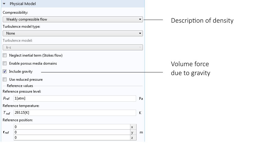
Settings window for the fluid flow interface showing the Weakly compressible flow option and gravity feature.
The figure below shows the flow between two vertically positioned circuit boards. Only the unit cell of one circuit board is shown in the figure. The second circuit board is placed just in front, with its back facing the board that is visible. The flow is completely driven by buoyancy; i.e., there is no fan.
The flow rate at the inlet is around 0.2 m/s and around 0.3 m/s at the outlet. There is no inlet of air from the sides, which means that the difference in flow rate is due to the expansion caused by the increase in temperature along the height of the channel between the circuit boards.
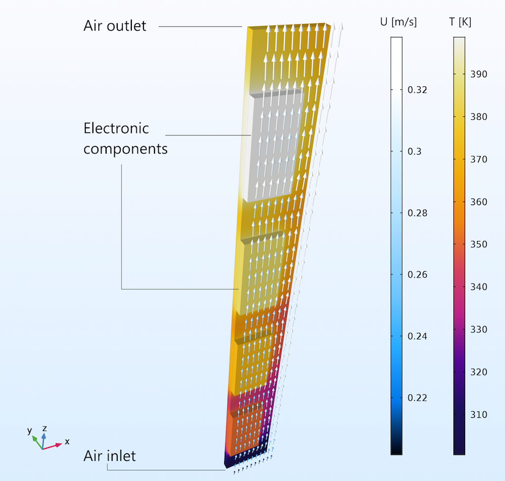
Buoyancy-driven flow between vertical circuit boards. The expansion is seen in the color legend for the arrows, where the flow velocity is around 0.2 m/s at the inlet and 0.3 m/s at the outlet.
Incompressible Flow with the Boussinesq Approximation
When the changes in density are negligible in terms of the influence of expansion on the velocity field, we can use the Incompressible flow option with the Boussinesq approximation for natural convection. This implies that the continuity equation is simplified even more than with the Weakly compressible flow option by treating the fluid as incompressible. In this case, the continuity equation becomes as follows:
(6)
Instead, a small change in density is accounted for in a volume force, which is introduced in the momentum equation in the opposite direction of gravity; by default, the z-direction. The small change in density is obtained by linearizing the fluid’s density at a reference temperature. The z-component of the volume force becomes as follows:
(7)
Where g is the gravity constant, \[{\rho _{{\text{ref}}}}\] is the density at a given reference temperature, α is the coefficient of thermal expansion of the fluid, and ΔT is the temperature difference measured against the reference temperature.
The advantage of using the Boussinesq approximation for buoyancy-driven flow is that the nonlinearities in the fluid flow equations are reduced and the problem becomes easier to solve numerically, requiring less iterations and allowing for larger time steps for time-dependent problems.
A typical example where the Boussinesq approximation can give a realistic description of the flow is for the modeling of liquid water subjected to relatively small temperature differences. The figure below shows natural convection in a glass of water heated from below. Here, we obtain a very complex flow pattern with an upward flow close to the middle and bottom of the glass and with downward flows between the vertical walls and the middle.
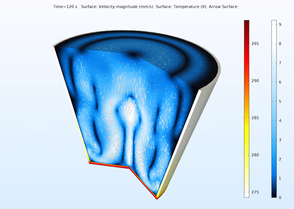
Natural convection in a glass of water. The plot shows the velocity field in the glass and the temperature distribution in the walls of the glass.
We can obtain the Incompressible flow option with the Boussinesq approximation for buoyancy-driven flow by selecting the settings shown in the figure below for the fluid flow interfaces in COMSOL Multiphysics.
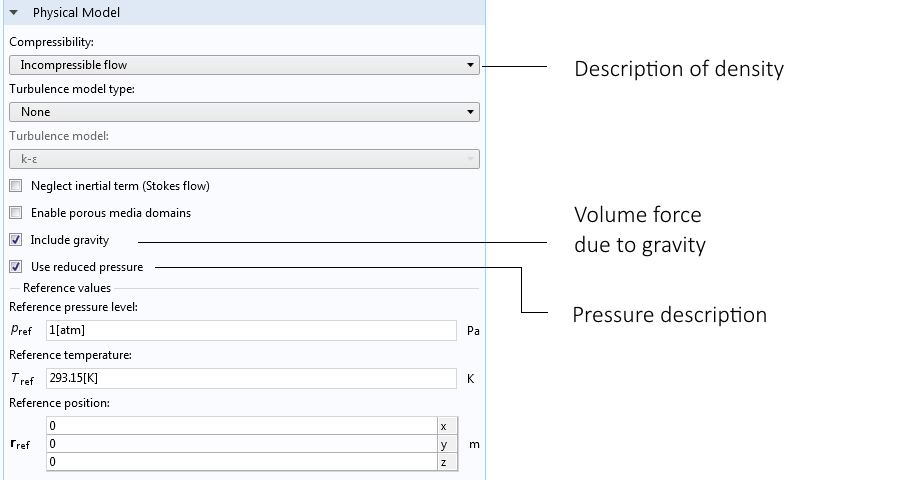
Selecting the Incompressible flow option, Gravity feature, and reduced pressure gives the Boussinesq approximation for a natural convection problem.
Constraining the Pressure Equation in Natural Convection Models
When modeling fully compressible flow, the pressure’s time dependency is included in the continuity equation, since density is a function of pressure for compressible fluids. This also means that it is usually sufficient to include an initial condition for the pressure in order to get a well-posed problem, even when we do not prescribe pressure at a boundary.
For weakly compressible and incompressible flows, the time-dependent pressure term in the continuity equation is neglected according to the discussions above. If there are no boundary conditions that set the pressure, the pressure field becomes undetermined, unless we set it in some point in the domain.
In COMSOL Multiphysics, we can use a so-called pressure point constraint in order to avoid an undetermined pressure field. The absence of a reference pressure point is often the source of problems with convergence when solving natural convection problems.
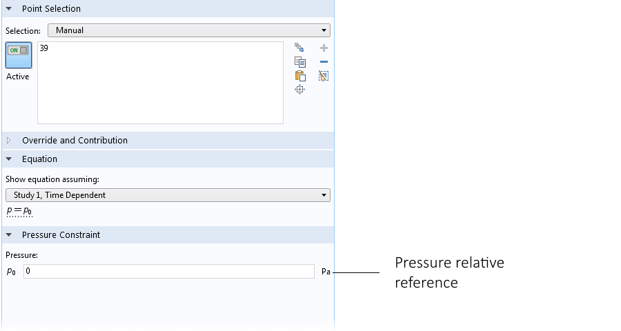
The settings for the pressure point constraint in the water glass example.
Solving Natural Convection Problems with a Coupled or Uncoupled Strategy
The equations that describe natural convection usually involve the momentum equation, the continuity equation, and the energy transport or mass transport equation. If buoyancy is driven by temperature differences, then the energy equation is fully coupled with the fluid flow equations (the Navier-Stokes equations). For natural convection, this coupling is fairly tight. This means that the most robust way to solve the equations is to use the fully coupled solver in COMSOL Multiphysics.
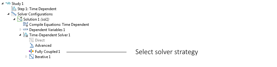
The solver branch in the model tree with the fully coupled solver option.
For very large problems, a segregated approach may be a preferable option. For example, if there are many chemical species and if buoyancy is caused by variations in density due to chemical composition, then a segregated approach may be the only viable option for getting decent memory consumption in the solution process.
Concluding Remarks
I would like to end this blog post with one more natural convection problem. I often think about natural convection when I smoke a cigar. Although I do not want to promote smoking, my favorite natural convection problem is the smoke from a cigar on a cold winter day. The figure below shows a lighted cigar resting on an ashtray with the flow distribution caused by the heat from combustion.
Natural convection (with a small forced component) around a lighted cigar resting on an ashtray.
Some of the flow caused by the lighted cigar is actually forced convection, since a large part of the tobacco goes to smoke, changing the density from around 500 to 1000 kg/m3 down to 1 kg/m3. This can be described as an inlet for the flow at the boundary between the ash and the air surrounding the cigar.
Further Reading
- Learn more about natural convection and fluid flow modeling on the COMSOL Blog:


Comments (8)
Saurav Chakraborty
November 25, 2017For using Boussinesq approximation with incompressible flow in natural convection , if we use the settings mentioned in this post in COMSOL 5.3, the material node does not ask for entering the value for the coefficient of thermal expansion. Also, there is no provision for entering the value of reference density in the physics node, the only values being asked are reference pressure and reference temperature. The equation section shows the body force term being formulated as (rho -rho.ref)*g, whereas it should have been [beta*rho.ref*g*(T-T.ref)]. This is quite ambiguous as to how COMSOL is calculating the body force. Please comment.
Mohamad Barekati Goudarzi
February 7, 2019Thanks Ed! This post was what I exactly needed.
Ali Asad
February 9, 2019Hello Ed
I wanted to know that while using the weakly compressible model, how is pressure being calculated as it has been ruled out of “equation of state” due to its weak dependence with density. Also please give an idea about how momentum equation is being handled with pressure terms present in them.
Ed Fontes
February 18, 2019Dear Ali,
The variables solved for in the Fluid Flow interfaces are the velocity vector (u, v, w) and the pressure p. The equation for the pressure is the continuity equation.
This means that p is used as the test-function in the weak formulation of the continuity equation. By default, the pressure solved for in the Fluid Flow interfaces (except for High Mach Number Flow) is the gauge pressure. Hence the absolute pressure p_A is obtained by adding a reference pressure p_ref to the gauge pressure, p_A = p_ref + p. For compressible flow, p_A is the pressure used in the equation of state, i.e. to determine the density. When using the weakly compressible option, p is assumed to be small relative to p_ref, and p_A can be approximated by p_ref in the equation of state.
In the solver, the momentum equation and the continuity equation are always solved together as a fully coupled system.
I hope this helps!
Best regards,
Ed
Fabio Pulvirenti
July 20, 2019Hello Ed
Is the cigar model available? Did you use a single phase flow and just considered buoyancy due to temperature differences? Would it be possible to apply a two-phase (smoke and air) non-isothermal flow?
Thanks
Fabio.
Diana Mora
June 20, 2023Hello Ed
Could you show me the derivation of equation 4 from the above equations.
Thanks
Ed Fontes
June 22, 2023 COMSOL EmployeeHi Diana,
I replied via support, since I could not upload my notes here.
Saludos,
Ed
Diana Mora
June 30, 2023Thank you Ed.
Could you send me the file of this COMSOL simulation?