

Measuring acceleration is important in high-speed dynamics, as velocity, force, and pressure are derived from it. Sensing elements inside accelerometers make it possible to obtain such measurements. As technology advances, these sensor packages must be optimized to handle higher vibrational frequency bandwidths. To accomplish this, researchers tested their novel piezoresistive sensor chip as part of a package design. Their simulation results, which agree well with experimental data, pave the way for optimizing sensor packages to achieve higher bandwidths.
Developing Sensors with Higher Bandwidths for Accelerometers
There are a number of industries that rely on accelerometers. Take automotive designers, for instance, who often use these electromechanical devices to analyze shock and vibrations in safety testing. In addition, the developers of consumer electronics use these devices as a means of detecting orientation in digital cameras and tablet computers.

Automotive safety testing is just one application of accelerometers.
To detect the size and direction of an object’s acceleration, accelerometers feature sensor packages. Together, the components of these packages determine the frequencies for which the accelerometer provides accurate measurements. For example, modern commercial products typically feature a bandwidth of 10 to 20 kHz. As technologies continue to evolve and higher frequencies need to be measured, sensor packages must be able to handle higher bandwidths.
Recognizing this, a team of researchers from the Fraunhofer Institute for High-Speed Dynamics, Ernst-Mach-Institut, EMI, and the Albert-Ludwigs-Universität Freiburg used the COMSOL Multiphysics® software to design and analyze a sensor package for a high-g accelerometer. At the heart of the design is a novel piezoresistive sensor chip, one that can measure transient accelerations up to 100,000 g. Compared to today’s state-of-the-art sensors, this piezoresistive sensor’s figure of merit (sensitivity multiplied by resonance frequency) is around an order of magnitude greater.
Using COMSOL Multiphysics® to Design and Analyze a Sensor Package for a High-G Accelerometer
To begin, let’s look at the design of the piezoresistive sensor chip. It includes:
- A stiff frame
- A bending plate
- Four piezoresistive elements, interconnected through a Wheatstone bridge
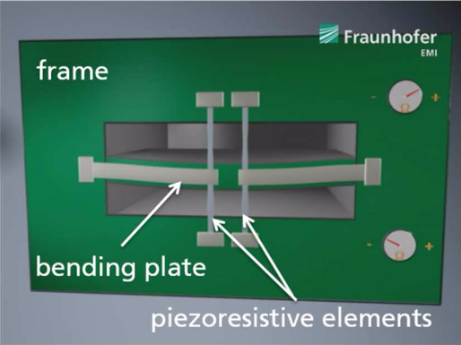
The sensor chip. Image by R. Langkemper, R. Külls, J. Wilde, S. Schopferer, and S. Nau and taken from their COMSOL Conference 2016 Munich paper.
In COMSOL Multiphysics, this configuration is fully modeled as a silicon MEMS device.
For the package itself, three of these chips are integrated onto a single ceramic plate. Oriented at right angles to one another, the chips are sensitive in the x-, y-, and z-directions.
The sensor — its package included — acts as a complex mass spring system. Bending in the plate as a result of acceleration causes the piezoresistive elements to stretch and compress, which in turn produces changes in electrical resistance.
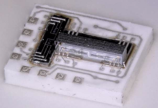
The complete sensor package. Image by R. Langkemper, R. Külls, J. Wilde, S. Schopferer, and S. Nau and taken from their COMSOL Conference 2016 Munich paper.
While the researchers tested multiple sensor package designs, we focus on one specific example here. The geometry for this sensor package, shown below, was imported into COMSOL Multiphysics® via LiveLink™ for Inventor®.
Each color represents the following:
- White: package box and cap
- Red: ceramic plate
- Gray: piezoresistive sensor chips
- Orange: grouting
- Green: adhesive layers
- Blue: cable dummy
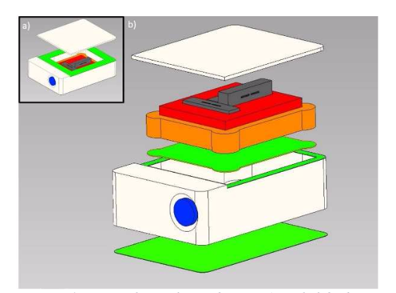
The example sensor package design with its cap lifted (a) and an expanded view (b). Image by R. Langkemper, R. Külls, J. Wilde, S. Schopferer, and S. Nau and taken from their COMSOL Conference 2016 Munich paper.
To analyze the sensor’s behavior over a specific frequency range, the researchers used two approaches:
- Modal analysis of the system
- Simulation of the sensor with an oscillating acceleration load applied between a frequency range of 0 to 250 kHz
The first approach provides the value and shape of the resonance frequencies, while the latter depicts the stress and displacement of components within the sensor package. This information is used to determine the relative resistance of the piezoresistive bridges as well as compute the output signals of the sensor chips.
Evaluating the Simulation Results
The simulation results shown here correspond to the following sensor package design parameters:
| Parameter | Setting |
|---|---|
| Wall thickness | 1 mm |
| Cap thickness | 200 µm |
| Package material | Titanium |
| Adhesive layer thickness | 20 µm |
| Adhesive Young’s modulus | 2.5 GPa |
| Sensor chip | Type M (0.65 µ V/V/g) |
Let’s look at the sensor’s output signal for the frequency range of 0 to 250 kHz. Note that this signal is computed for 100,000 g and a supply voltage of 1 V. Further, a limit of 5% is defined with regards to the sensor’s maximum change in sensitivity.


Output signal for the sensor at various excitation frequencies. The plot on the left shows the whole frequency spectrum, while the plot on the right shows a close-up view of 0 to 100 kHz. Images by R. Langkemper, R. Külls, J. Wilde, S. Schopferer, and S. Nau and taken from their COMSOL Conference 2016 Munich paper.
From the plot on the left, it initially appears that the curve’s behavior is flat until about 130 kHz. But with a closer view, shown in the plot on the right, the sensitivity changes are also visible at lower frequencies. With the 5% limit in place, the potential bandwidth of the sensor package is 47 kHz.
The sensor package modes are also analyzed, specifically those shown as peaks in the frequency spectrum. As highlighted in the previous plot, the first mode, or “cap mode”, occurs at 39 kHz and has minimal influence on sensitivity. Aside from the cap oscillations, the first mode, or “package mode”, occurs at 128 kHz. This mode, which is also highlighted above, has a significant effect on the output signal.
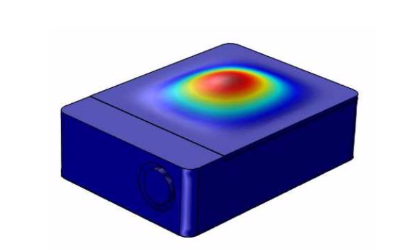
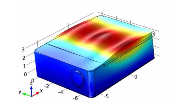
Left: The first cap mode, deflecting in the z-direction. Right: The first package mode, oscillating in the y-direction. Images by R. Langkemper, R. Külls, J. Wilde, S. Schopferer, and S. Nau and taken from their COMSOL Conference 2016 Munich paper.
From the modal analysis, an additional oscillation is observed at 287 kHz. As the main source of displacement for the sensor element, this mode is expected to have the most influence on the sensor’s signal. To test this assumption, the researchers turned to experimental tests.

Main displacement mode inside the sensor element. Image by R. Langkemper, R. Külls, J. Wilde, S. Schopferer, and S. Nau and taken from their COMSOL Conference 2016 Munich paper.
Verifying Results with Experimental Data
When adapting the simulation study to the experimental phase, the researchers used the following parameters. For practical reasons, these parameters differ slightly from those used in the model.
| Parameter | Setting |
|---|---|
| Wall thickness | 1 mm |
| Cap thickness | 200 µm |
| Package material | Titanium |
| Adhesive layer thickness | 20 to 70 µm |
| Adhesive Young’s modulus | 0.56 GPa |
| Sensor chip | Type L (1.3 µ V/V/g) |
An additional simulation study helped to predetermine the ranges of expected frequencies:
- 5% limit: 16 to 30 kHz
- Package mode: 67 to 98 kHz
- Sensor element mode: 129 to 200 kHz
In the experiment, a small glass hammer stimulates the sensor oscillation in order for the researchers to measure the eigenfrequencies. A sampling rate of 10 MHz is used to record the sensor’s impulse answer.
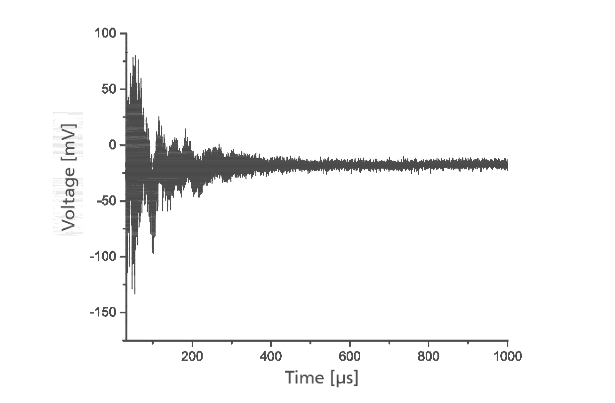
Impulse answer of the sensor to an oscillation. Image by R. Langkemper, R. Külls, J. Wilde, S. Schopferer, and S. Nau and taken from their COMSOL Conference 2016 Munich paper.
To examine the impulse answer for relevant frequencies, the signal is converted into the frequency domain. As indicated below, multiple peaks appear at higher frequencies. The highest peak at 930 kHz represents the first eigenfrequency of the actual sensor chip. The lower frequencies, up to about 70 kHz, are a portion of the excitation impulse.


Left: Impulse answer of the sensor from 0 to 2 MHz. Right: Impulse answer of the sensor from 0 to 350 kHz. Images by R. Langkemper, R. Külls, J. Wilde, S. Schopferer, and S. Nau and taken from their COMSOL Conference 2016 Munich paper.
Something interesting to note is the peak that appears at 153 kHz. This represents the sensor element’s oscillation that is expected between 129 and 200 kHz. This finding supports the theory that this oscillation has the biggest influence on the sensing element.
In the sensitivity analysis, an acceleration of 8600 g is applied to each axis. A titanium Hopkinson bar is used to produce the shock load, with an attachment included to ensure equal distributions of the load on each sensor axis.
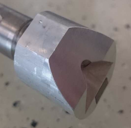
The attachment for the Hopkinson bar. Image by R. Langkemper, R. Külls, J. Wilde, S. Schopferer, and S. Nau and taken from their COMSOL Conference 2016 Munich paper.
The measured output signals, shown in the plot below, are used to compute the sensitivities of the different axes. The expected sensitivity is 1.3 µ V/V/g, with a potential maximum deviation of 30%. The greatest deviation in sensitivity occurs at the x-axis (around 23%), while the other axes have much lower percentages. Note that all of the sensor chips fall within this deviation range.
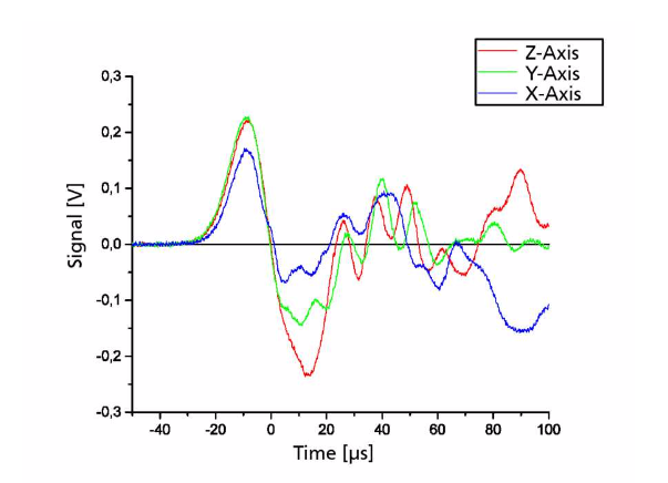
The measured output signals under a load of 8600 g. Image by R. Langkemper, R. Külls, J. Wilde, S. Schopferer, and S. Nau and taken from their COMSOL Conference 2016 Munich paper.
These findings show good agreement with the expected values from the simulation results, further highlighting the suitability of the sensor package design for a high-g accelerometer.
Learn More About Analyzing and Optimizing Sensor Designs
- Read the full COMSOL Conference paper:
- Explore the role of simulation in analyzing and improving other sensor designs:
Autodesk, the Autodesk logo, and Inventor are registered trademarks or trademarks of Autodesk, Inc., and/or its subsidiaries and/or affiliates in the USA and/or other countries.


Comments (2)
Awatef khlifi
November 29, 2019I am working in piezoresistive accelerometer and i am trying to make a package. Can i get the comsol guide or comsol file for this work
Brianne Christopher
December 2, 2019Hello Awatef,
Thank you for your comment.
For questions related to your modeling, please contact our Support team.
Online Support Center: https://www.comsol.com/support
Email: support@comsol.com