

Have you ever used your hands to make shadow puppets on the wall? By shining a light behind your (three-dimensional) hands, you create two-dimensional projections on the wall. When analyzing your simulation data in COMSOL Multiphysics, you can do something similar with your model using projection operators.
2D Axisymmetric Pipe Flow Model Example
Suppose you have just computed the solution of your 2D axisymmetric pipe flow model with a chemical species, c, transported by the flow. You are looking at the spatial distribution of the concentration in the pipe and you notice that the concentration decreases in the direction of the flow. While you can clearly see this trend qualitatively in the surface plot below, you may want to put it in more quantitative terms.
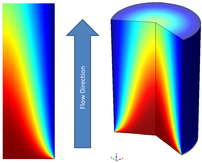
Concentration and flow direction.
One way of achieving this is to plot the average concentration for every cross section along the axis of the pipe. In COMSOL Multiphysics, you use projection operators to do just that.
Projection Operators, Reducing the Source Dimension by One
Let’s revisit our shadowgraphy analogy and think about how that works, conceptually. When you place your hands between a light source and a wall, your hands obstruct the light path, and you can see a shadow on the wall, i.e. a 2D image of your 3D hands.
You can think of projection operators in the COMSOL software as a tool to make “shadow puppets” of your model. The model (or a part of it) takes the role of the hands. This is called the source in the operator settings. The wall in this analogy is another part of the model: the destination. This is where the shadow is formed.
Just like shadow puppets, the result of a projection in COMSOL Multiphysics reduces the dimensions of the source by one. The “image” is formed by integrating an expression in the “direction of light”. This direction is specified by a map between the source and the destination. Here you have two choices: the Linear Projection for linear maps and the General Projection for more complex situations. Let’s use these to plot the average cross-sectional concentration along the axis of the pipe we introduced above.
Linear Projection
Let’s assume you are interested in the average species concentration, c_{av}(z), in a cross section at height z along the axis of the flow channel. Since you have a 2D axisymmetric geometry, the cross sections are represented by horizontal lines and the average can be computed with the following integral:
Here, A(z)=\pi\cdot R(z)^2 is the cross section area and R(z) is the length of the integral, which in this example is equal to the radius of the pipe.
In the COMSOL software, the line integrals shown here can be solved with a Linear Projection operator. From the discussion above, you know that you need a Source, Destination, and a map between the two to set up the operator. When you add a Linear Projection to the Definitions of your component, you first select the geometry entities that belong to the Source.
In our pipe example, this is the entire model domain 1. The Linear Projection uses linear maps that are defined by lines between vertices that you select. You are now ready to set up the map, starting with the Destination. Here, this should be the axis of the flow channel, thus you select Destination vertices 1 and 2 accordingly. Next, select the line in the Source that corresponds to the Destination. In this scenario, that is the same line, therefore you assign the same points to Source vertices 1 and 2. The Source has one more vertex than the Destination. This is used to specify the direction for the line integrals. In our example, you select Vertex 3 here, which means that the line integrals are computed parallel to this line as indicated by the white arrows in the figure below.
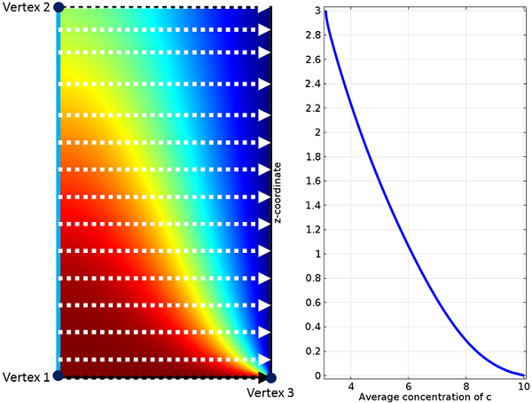
Concentration with arrows representing the line integrals and the resulting average concentration of the chemical species, c.
To summarize, the first axis (between vertices 1 and 2) contains the starting points of the line integrals, while the second axis (between vertices 1 and 3) gives the direction of integration.
You can now use the operator (called “linproj1” by default) to integrate the concentration of c and divide it by the length of the integral to get the average concentration. If the length R(z) is not constant or unknown, it can be evaluated by the operator as well. Here is the resulting equation:
To plot the result, use a 1D Line Graph with linproj1(c*2*pi*r)/linproj1(2*pi*r) as the expression and the left boundary as the selection.
General Projection
You may also set up the average with the General Projection operator. As the name suggests, this operator can handle more complex maps and can, for example, use path integrals in any (curved) direction of its domain. You can, of course, also use the General Projection operator to set up a Linear Projection. That option is relevant when you do not have vertices in your model geometry to adequately set up the Linear Projection operator. In this situation, you can either modify the geometry to include the necessary vertices, or you can use the General Projection operator, where you define the map between Source and Destination directly with mathematical expressions.
To get a better understanding, let’s have another look at the 2D axisymmetric example model. After adding the General Projection to the component’s Definition section, you again first select the Source geometry. The operator’s settings contain a field for mathematical expressions defining the Source Map and the Destination Map. In our example, the expressions are linear functions of the coordinates. If you again start with the Destination, you enter the flow axis, i.e. the z-axis, in this geometry. Since you use the same line in the Source, the x-expression there is the z-axis as well. The y-expression defines the direction of integration, which in this case is the r-axis. You can now use the General Projection operator (called “genproj1” by default) to obtain the same results as with the Linear Projection before.
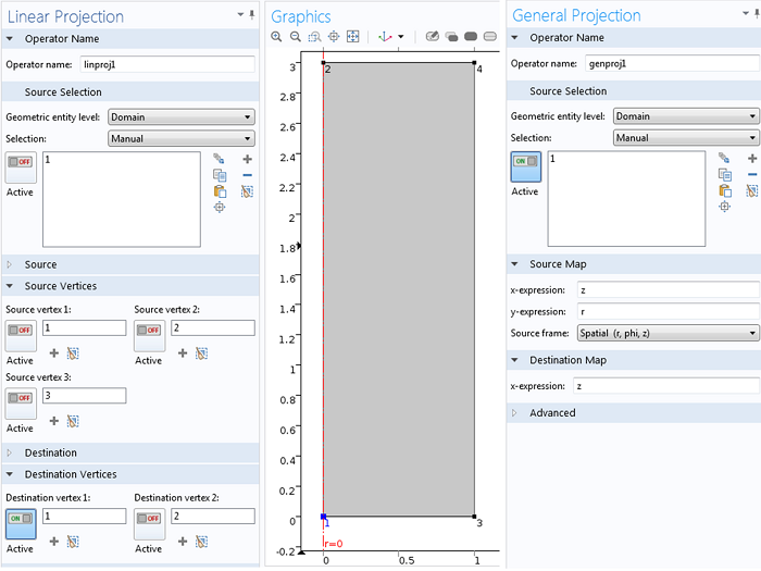
Settings of the Linear and General projection operators.
Projecting More than One Dimension
What if you have a 3D version of your model, perhaps due to an asymmetric concentration distribution? In this case, you can compute the average for each xy cross section by computing the following double integral over x and y:
where A(z) is the cross section area.
In COMSOL Multiphysics, you can evaluate this double integral by using two projection coupling operators. The first operator projects from 3D to 2D by integrating over x (the y-direction would work equally well here). The second operator projects the results of the first from 2D to 1D by integrating over the remaining coordinate.
It is easiest to set up the operators if the geometry contains the planar face in the yz-plane. If this is not the case, you have at least three options: you can modify the geometry of the component, but you then have to recompute the solution, which is not a convenient option if the model takes a long time to compute; you can use a General Projection operator instead; or you can add another component with a 2D geometry for the plane and project from the 3D component to the 2D component, which may be the easiest option. This works because Source and Destination do not have to belong to the same model component. If you go with the third option, you can run an update to your solution and avoid having to recompute everything.
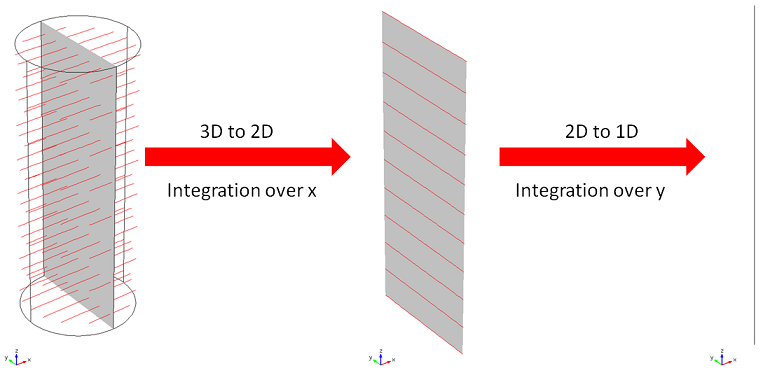
The double integration is performed by two projection operators. The red lines represent the lines integrated over.
Concluding Remarks
Here, we have demonstrated how to use projection operators to analyze simulation data. When applicable, this technique can be useful to distill the essence of your results and help you gain deeper insight into the underlying physics. If you are interested in learning more about using projection operators, please contact us.

Comments (2)
Evgeni Sergeev
May 22, 2014Thanks, this was very helpful. I would add that the figure “About Source and Destination Mappings” in the documentation article “Model Couplings” is essential to understanding General Projection operators.
Is it possible to project the maximum or minimum instead of integrating in one direction?
Clemens Ruhl
May 26, 2014Dear Evgeni,
That’s true; in the documentation are additional helpful information.
In this case you do not need the projection operator. This can be done with a maximum operator in combination with the dest operator. The latter is used in limiting the max evaluation to the slice in which e.g. x = dest(x) +/- dx. Here dx is a defined parameter for the width of the slice which should be not too small in comparison with the mesh size. In practice you are probably better off slicing up the actual geometry and evaluating the maximum on each slice.
Best
Clemens