

The goal of mesh adaptation is to modify the mesh to solve a problem more efficiently. We want to use as few elements as possible to obtain an accurate solution. Typically, we would like a coarser mesh in regions that are not very important and a more refined mesh in regions of interest. We might even consider anisotropic elements. As of version 5.4, the COMSOL Multiphysics® software includes enhanced tools to adapt a mesh. Let’s take a look.
Knowing Your Mesh Element Size
To adapt a mesh, it is necessary to provide the desired element size. Finding the right size is not an easy task. In fact, it is subject to a lot of research. In COMSOL Multiphysics, you can use the Adaptation and Error Estimates functionality in the study (for stationary and eigenvalue problems) to automatically adapt the mesh based on built-in error estimates.
Mesh adaptation in COMSOL Multiphysics, though, is not limited to using built-in error estimates: It is much more flexible. It’s possible to solve a simpler problem on a coarse mesh and then evaluate an expression on that solution to control the element size for the more advanced problem. You could also use an imported interpolation function or any expression you can come up with.
This blog post does not delve into this aspect but instead assumes that you, implicitly or explicitly, know your desired element size as a function of x, y, and (in 3D) z. What does this mean? The interpretation is that the length of an edge of a mesh element is given by the function evaluated at the midpoint of that edge. Naturally, it is (in general) impossible to satisfy this requirement exactly. Even a single triangle needs to satisfy the triangle inequality. But it is important to keep this picture in mind: The size expression represents the desired element edge length at each point in space.
2 Methods for Adapting a Mesh to a Size Function
In COMSOL Multiphysics, while working from the Mesh node, there are two fundamentally different ways to construct a mesh adapted to a size function. You can use the Size Expression attribute in the meshing sequence to influence the sizing used when generating a mesh. If you use automatic adaptation from a study, this corresponds to the Rebuild mesh option. The free mesh generators (Free Triangular, Free Quad, and Free Tetrahedral) take this sizing into account. On the other hand, structured methods such as Mapped and Swept (and to some extent, Boundary Layers) ignore the size expression attribute. (By definition, a structured mesh cannot respect a varying size field.) In short, if you build a structured mesh, you probably shouldn’t use this method.
The other method is to use the Adapt operation. This operation modifies an existing mesh by element refinement and coarsening. You can use the Adapt operation on a mesh with any element type and also on imported meshes. It is a more powerful (you might even call it “brutal”) method and may respect the specified size expression better. However, the result is generally not as smooth as when the mesh is generated from scratch.
Let’s take a closer look at these two methods and see how the results differ.
Using the Size Expression Attribute
As mentioned, an advantage of this method is that you often get high-quality meshes. But it might not respect the desired size if it leads to low-quality elements (which is often the case for rapid size transitions). For a discussion on what quality means for a mesh, see, for example, the blog post “How to Inspect Your Mesh in COMSOL Multiphysics®“. Since the mesh is built from scratch for each adaptation, the process can be time consuming for complex geometries.

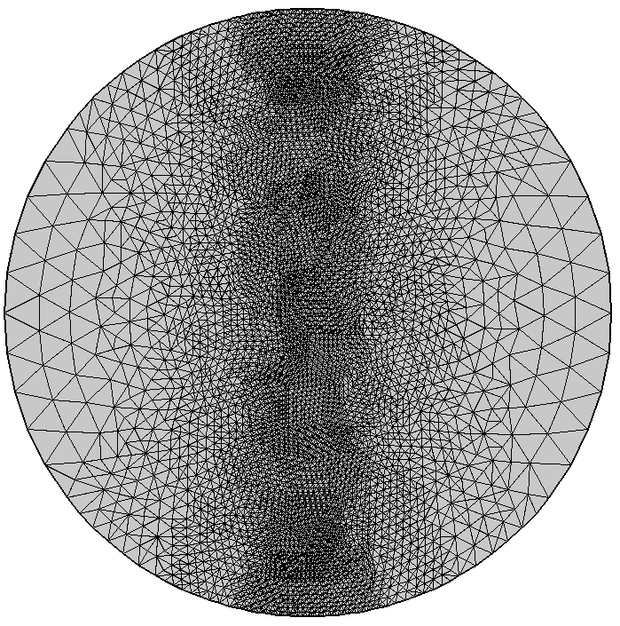
The Size Expression attribute is used to apply a size expression to the triangular mesh on a circle. Note the high-quality elements and the smooth size transition.
If you have a known size expression (for example, a global interpolation function), it is often convenient to evaluate on a background grid. (Evaluate on: Grid in the picture above). Make sure that the grid resolution is sufficiently high to capture all of the features in your size expression.
When the size expression depends on a known spatially varying quantity, such as the materials, you can use the Initial expression evaluation option. Then, it is possible to use any expression from the model. The expression is evaluated as it would be prior to solving (compare the Get Initial Value for Step command, available for a study step). You may also specify a certain study step, as the value of some expressions depends on the study.
Finally, you can also evaluate on an existing solution. The Error Indicator type of expression is used for the built-in Error estimates, but you can also use any size expression — which may depend on the existing solution. Sometimes, you might want to refine the mesh where the stress is large.
Using the Adapt Operation
The other alternative is to start with an existing mesh and modify it to match the desired size. This is what the Adapt operation does. It is available in all dimensions and also works for imported meshes. Many of its options and input fields are the same as for the Size Expression attribute.
There are three adaptation methods: Longest edge refinement, Regular refinement, and General modification. The two refinement methods are based on the bisection of element edges that are too long. All existing mesh vertices are kept, so the mesh cannot be coarsened by these methods. The General modification method is available as of version 5.4 of COMSOL Multiphysics. As the name suggests, it can modify the mesh in a very general way:
- Elements can be refined
- Vertices can be deleted to coarsen the mesh if it is too fine
- Elements can be modified and mesh vertices can be moved to improve the quality

The same size expression as for the Size Expression attribute is applied using the Adapt operation with General modification. While the element quality is sufficiently high for most purposes, the size transition is not as smooth as when the mesh is generated from scratch.
If you change the adaptation method to Longest edge refinement, the result is instead as shown below. Too-long edges are bisected until the mesh is sufficiently refined. This mesh operation is very fast, but the method will generally produce elements of low quality, even when the input mesh is of high quality.
Same model as above, but with the adaptation method set to Longest edge refinement. Here, you can see patterns resulting from the shape of the original triangles.
Supporting All Element Types
The Adapt operation can be used on meshes with all element types and works on domains with structured mesh (although, the mesh will generally not be structured after adaptation). We need to be careful, though, when using this method on nonsimplex elements (quadrilaterals in 2D and hexahedra, prisms, or pyramids in 3D), since the result may be poor. Let’s take a look at how size transitions are treated in such cases. In 2D, triangles are inserted in the quad mesh in regions of size transition.
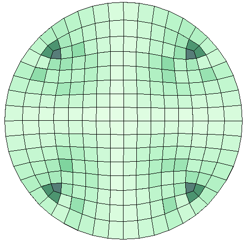
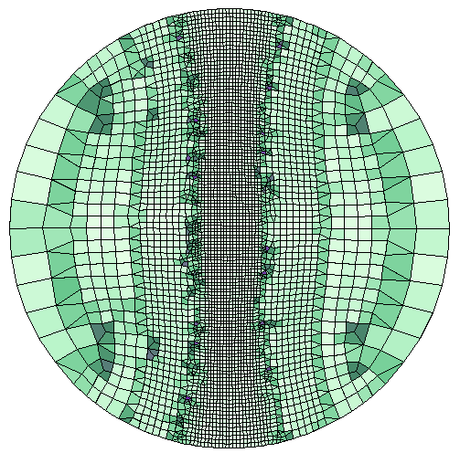
Left: The default Free Quad mesh of a circle. The elements are colored by maximum angle quality. Right: The result after adaptation to the same size expression as above. Note how triangles are used in the size transition zones.
In 3D, tetrahedra and pyramids are typically used for the size transition region, although other element types may also be inserted when suitable. The following image shows a cylinder with a coarse hexahedral mesh, which is adapted with the expression 0.02 + z*z.
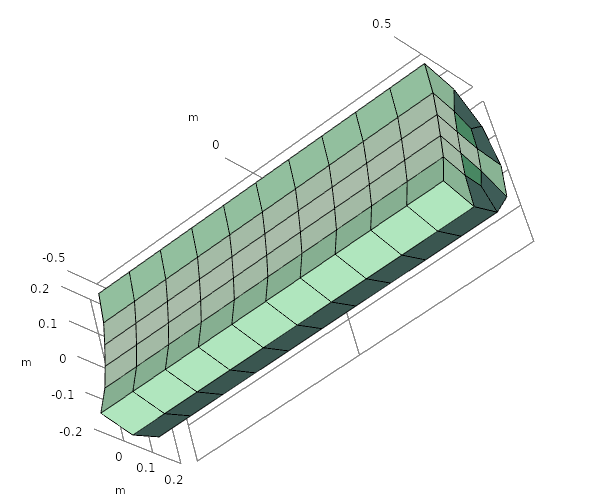
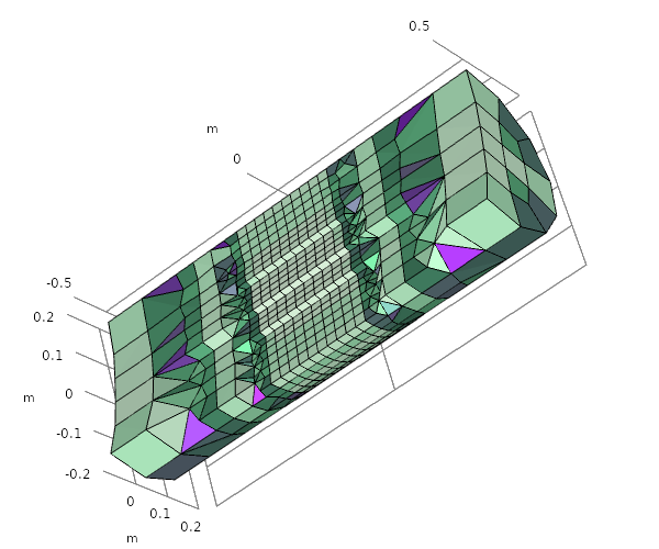
A meshed cylinder before and after adaptation.
Mesh Adaptation for Boundary Layer Meshes
In all of the examples above, the specified size functions represent the isotropic element size; that is, all edges of an ideally shaped element have (approximately) the same length. If the mesh you need to adapt is anisotropic (for example, a boundary layer mesh where the elements are stretched along the boundary) the adaptation will modify it toward an isotropic mesh. The boundary layer elements may even be completely deleted! This is not the desired result. A workaround is to disable coarsening. Then, the boundary layers will be kept.
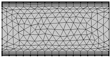
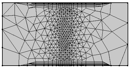
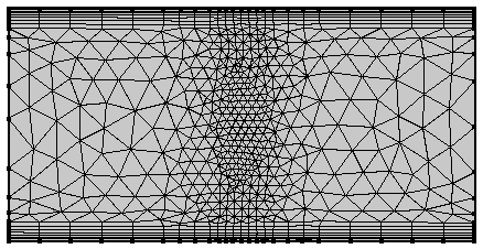
Left: A rectangle, centered at the origin, with a boundary layer mesh. Middle: Adaptation, by General modification, to the size expression 0.04 + x*x. The boundary layer is deleted by the coarsening operation. Right: The result of the adaptation with disabled coarsening. The boundary layers are kept.
Constructing Anisotropic Meshes
The Adapt operation can also be used for anisotropic adaptation. Let’s take a quick look at this fairly advanced topic. An anisotropic mesh element is an element where the ideal element is stretched in some direction. Such meshes are common in CFD computations, the boundary layer mesh being a prominent example. To adapt anisotropically, select Anisotropic metric as the type of expression. You then need to specify a 2×2 (in 2D) or 3×3 (in 3D) symmetric matrix. The interpretation is as follows: The vector representing an edge of an element is transformed by the matrix in that point, and the length of the transformed vector is measured. If the length is shorter than 1.0, it is considered too short. If it is longer than 1.0, it is considered too long. This measure is used to control the adaptation. The images below demonstrate how this approach can be used.
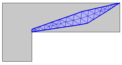
A mesh control domain is meshed with triangular elements.
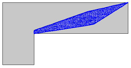
Anisotropic adaptation is applied. The metric in this case is specified by the constant matrix \begin{pmatrix}10 & -10 \\-10 & 60\end{pmatrix}.
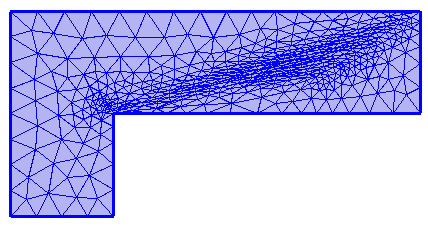
The surrounding domain is meshed by a Free Triangular operation.
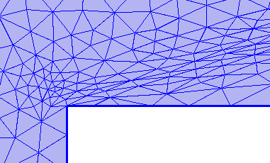
The mesh control domain is merged into the larger domain.
Concluding Remarks
We have shown how the mesh adaptation tools in COMSOL Multiphysics can be used to construct meshes adapted to a specific purpose. The Size Expression attribute in the Mesh node can be used to control the size used when generating triangular and tetrahedral mesh. The result will often be smooth and of high quality. Another option is to use the Adapt operation, which modifies an existing mesh. It is a powerful tool that can modify any type of mesh and generate anisotropic mesh elements.
Next Steps
Learn more about how COMSOL Multiphysics can suit your modeling needs by contacting us to evaluate the software:
Further Resources
- Learn more about creating meshes on the COMSOL Blog:
- Check out these related tutorial models:

Comments (0)