

Graphene can be created by way of thermal decomposition at high vacuum. In order to design and optimize these high-vacuum systems engineers might look to simulation, but there are currently not many modeling tools that are up to the task. Let’s have a look at how vacuum systems are relevant to graphene production, why you should simulate them, and how.
Obstacles in Bringing Graphene to the Masses
A while back I blogged about graphene and some of its properties, as well as some of the modeling tools available in the COMSOL Multiphysics® software for investigating applications of this exotic material. One of the main hurdles to overcome before graphene can be released to the mass market is how to manufacture it in an economical way. Many production methods are currently employed, including exfoliation, expitaxial growth on a suitable substrate, reduction of graphene oxide, pyrolisis or growth from metal-carbon melts.
In this thesis titled “Growth of Graphene Films on Pt(111) by Thermal Decomposition of Propylene“, the author explains how graphene can be manufactured using thermal decomposition at high vacuum. As my colleague Bjorn mentions in his blog post on “What Is Molecular Flow?” there are few modeling tools available to assist with design and optimization of high-vacuum systems, especially if the system is nonisothermal. Gases at low pressures cannot be modeled with conventional fluid dynamics tools because kinetic effects become important as the mean free path of the gas molecules becomes comparable to the length scale of the flow. The pressure on surfaces depends primarily on the line of sight with respect to molecular sources and sinks in the vacuum system. The nonisothermal vacuum system described in the thesis would inevitably be expensive to build, so any design optimizations that could be made before construction would result in big savings further down the line. Some estimations on the fluxes onto surfaces and deposition rates are given in the thesis, but these don’t take into account the geometry of the system, the fact that different surfaces have different temperatures, or the location of the pumps.
Soon You Can Model High-Vacuum Systems
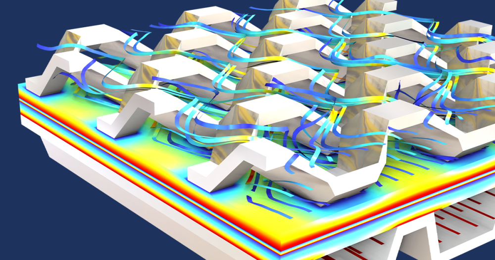
We at COMSOL are getting ready to announce that a dedicated product for modeling high-vacuum systems, the Molecular Flow Module, will be made available to our customers in early May. The product will greatly expand upon the capabilities currently available in the Microfluidics Module. The Molecular Flow Module is a collection of tailored physics interfaces for the simulation of kinetic gas flows. The module includes two physics interfaces: the Transitional Flow interface and the Free Molecular Flow interface. The Transitional Flow interface uses a discrete velocity/lattice Boltzmann approach to solve low-velocity gas flows in the transitional flow regime. The Free Molecular Flow interface uses the angular coefficient method to compute the particle flux, pressure, and heat flux on surfaces. The number density can be computed on domains, surfaces, edges, and points and is thus available to be coupled to other physics.
Editor’s note: The Molecular Flow Module was released on May 3, 2013.
Why Simulate Vacuum Systems?
Simulations can increase the pace of product development and also lead to a better understanding of vacuum systems for design engineers. High and ultrahigh vacuum systems are typically very expensive to construct and test. It is not only the cost to design and machine parts; a large amount of time can be spent baking out, pumping down, and checking for leaks in the system. Imagine if a smaller pump could be fitted onto a process tool simply by placing the pump port at a specific location. Or that the chamber met the necessary specification on the first build. The cost savings would be substantial. The Molecular Flow Module will allow you to test and optimize different designs before you have to start cutting metal.
Applications Relevant to Vacuum Processing and Graphene Production
In order to accurately model nonisothermal molecular flows and deposition rates onto substrates on arbitrarily complicated geometries, a sophisticated modeling approach is required. Since gas molecules interact with surfaces more frequently than they interact with one another, the flow of gas is determined by collisions with the surfaces in the system. It becomes necessary to solve a complicated integral equation in order to compute the molecular flux, pressure, heat flux, and number density in the system. The molecular flux can be used in combination with a suitable differential equation to determine the deposition rate and the deposited film thickness as well.
Let’s have a look at a couple of modeling examples.
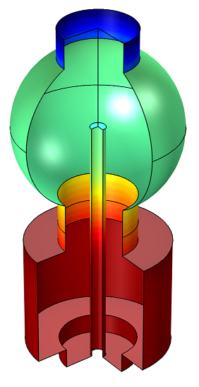
Example 1: Compute the Thickness of a Thermally Evaporated Gold Film
Gold is evaporated from a thermal source at a temperature of 2000 K onto a substrate held on a fixed surface. The deposited film thickness on the substrate and the chamber walls is computed.
Molecular flow calculations can show uniformity and deposition rate onto a wafer from a thermally evaporated material.
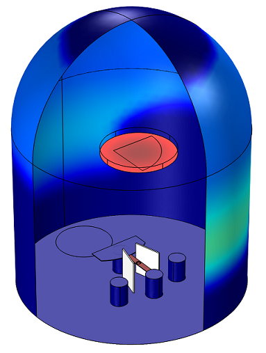
Example 2: Adsorption and Desorption of Water in a Load-Lock Vacuum System
The system consists of two chambers separated by a gate valve (not shown in the plot below). The lower cylindrical chamber is the load lock chamber. The upper spherical chamber is a high-vacuum chamber, which is not vented during the sample-loading process. The vacuum pump is located opposite the gate valve and has a constant speed of 500 l/s.
Time-dependent adsorption and desorption of water in a vacuum system at low pressures. The water is introduced into the system when a gate valve to a load lock is opened and the subsequent migration and pumping of the water is modeled.

Comments (3)
Sébastien Desaulle
May 23, 2018Hi Dan,
I hope you’re doing well. Could you please tell what temperature you would consider for the Knudsen number calculation in the gold evaporator model? I would choose the gold bath free surface temperature. Is this correct? Many Thanks.
Best regards,
Sébastien
Daniel Smith
May 23, 2018Hi Sebastien, I think the way to compute the Knudsen number in that specific model is to compute the number density at a point between the evaporator and the wafer, then use the fact that the mean free path is:
lambda = 1/(N*sigma)
where N is the number density and sigma is the collision cross section. Using N=1.6E17[1/m^3], which I got by inserting a point in the geometry at (0,0,200[mm]), and a rough cross section of sigma=9E-20[m^2], the mean free path comes out to be around 70[m]. For a characteristic length of around 280[mm] (distance between the source and target) I get a Knudsen number of 250, which is well in the molecular flow regime.
Sébastien Desaulle
May 23, 2018Hi Dan,
Thank you very much for your fast and detailled answer! This will be very helpful!
I wish you a nice day.
Best regards,
Sébastien