

We all know that COMSOL Multiphysics can take partial derivatives. After all, it solves partial differential equations via the finite element method. Did you know that you can also solve integrals? That alone shouldn’t be very surprising, since solving finite element problems requires that you integrate functions. The COMSOL software architecture allows you to do a bit more than just evaluate an integral; you can also solve problems where you don’t know the limits of the integral! Here’s how.
Integrating a Function
Consider the problem of taking the integral of a quadratic function:
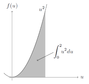
The integral is the area of the shaded region.
We can evaluate this integral within COMSOL Multiphysics by using the integrate function, which has the syntax: integrate(u^2,u,0,2,1e-3). Here, the first argument is the expression, the second is the variable to integrate over, the third and fourth arguments are the limits of the integration, and the optional fifth argument is the relative tolerance of the integral, which must be between 0 and 1. If the fifth argument is omitted, the default value of 1e-3 is used. We can call this function anywhere within the set-up of the model.
Here, we’ll use it within the Global Equations interface:
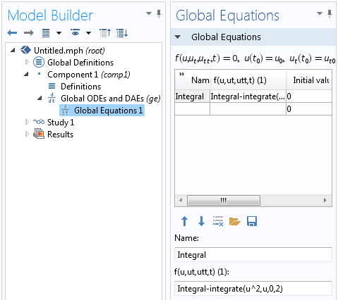
The Global Equation for Integral computes the integral between the specified limits.
There aren’t any big surprises here, so far. We can solve this problem in COMSOL Multiphysics or by hand. But suppose we turn the problem around a bit. What if we know what the integral should evaluate to, but don’t know the upper limit of the integral?
Let’s look at how to solve the following problem for the upper limit, u_b:
We can solve this by changing the Global Equation such that it solves for the upper limit of the integral:
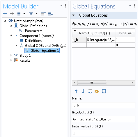
The Global Equation for u_b solves for the upper limit of the interval for which the integral evaluates to 6.
There are a few changes in the above Global Equation. The variable is changed to u_b and the expression that must equal zero becomes: 6-integrate(u^2,u,0,u_b). So, the software will find a value for u_b such that the integral equals the specified value.
Note that the initial value of u_b is non-zero.
Since we use the Newton-Raphson method to solve this, we should not start from a point where the slope of the function is zero. After solving the problem, we find that u_b = 2.621.
Now, let’s complicate things a bit more and solve the following problem for both limits of the interval, u_a and u_b:
Since we have two unknowns, we clearly need to have one more equation here, so let’s additionally say that (u_b-u_a)-1=0
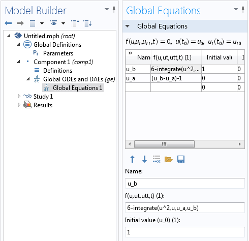
An additional equation is added to specify the difference between the upper and lower limits of the interval.
Solving the model, shown above, will give us values of u_a = 1.932 and u_b = 2.932. It would actually also be possible to solve this with a single Global Equation, by writing 6-integrate(u^2,u,u_b-1,u_b) as the equation to solve for u_b, but it is interesting to see that we can solve for multiple equations simultaneously.
An Example From Heat Transfer
Next, let’s put the above technique into practice to determine the operating conditions of a heat exchanger. Consider the Model Library example of the geothermal heating of water circulating through a network of pipes submerged in a pond.
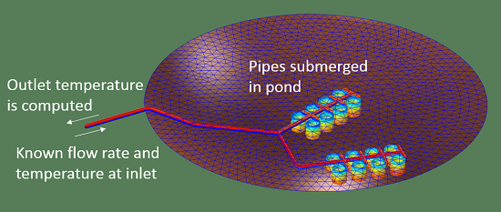
Water pumped through a submerged network of pipes is heated up.
In this example, the Pipe Flow Module is used to model water at 5°C (278.15 K) pumped into a network of pipes and heated up by the relatively warmer water in a pond. The temperature of the water in the pond varies between 10°C and 20°C with depth. The computed temperature at the output is 11.1°C (284.25 K). If the mass flow rate of water is specified to be 4 kg/s, then the total absorbed heat is:
where \dot m is the mass flow rate and C_p(T) is the specific heat, which is temperature dependent.
Now, in fact, the network of pipes we have here is a closed-loop system, but we simply aren’t modeling the part of the system between the pipe outlet and inlet. This model contains an implicit assumption that as the water gets pumped from the outlet back to the inlet, it is cooled back down to exactly 5°C.
So, instead of assuming that the temperature of the water coming into the pipe is a constant temperature, let’s consider this closed-loop system connected to another heat exchanger that removes a specified amount of heat. Suppose that this heat exchanger can only extract 10 kW. What will the temperature of the water in the pipes be?
Clearly, the first step here would be to write the integral for the extracted heat, in terms of the unknown limits, T_{in} and T_{out}:
The second condition that we need to include is the relationship between the input and output temperatures. This is computed by our existing finite element model. The model uses a fixed temperature boundary condition at the pipe inlet and computes the temperature along the entire length of the pipe. Therefore, all we need to do is add a Global Equation to our existing model to compute the (initially unknown) inlet temperature, T_in, in terms of the extracted heat, and the temperature difference between the inlet and outlet.
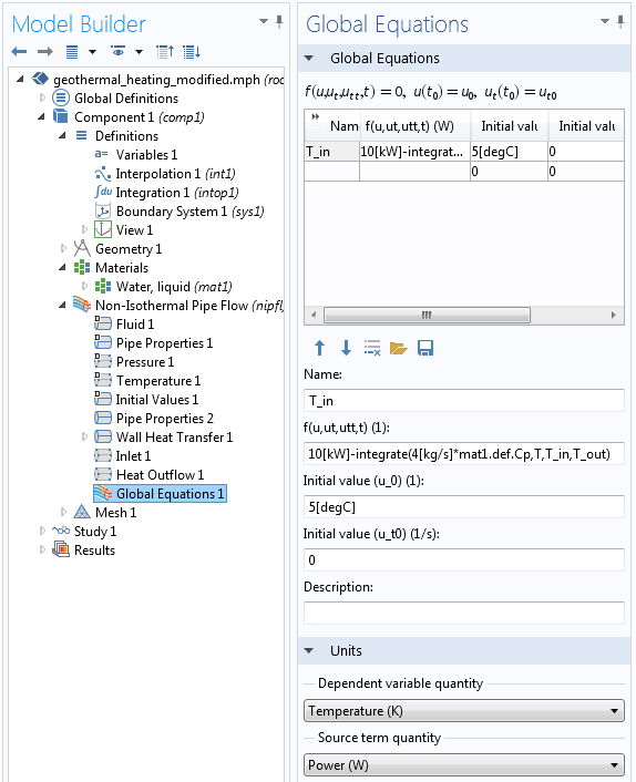
The Global Equation that specifies the total heat extracted from the pond loop.
Let’s look at the equation for T_in, the inlet temperature to the pipe flow model, in detail:
10[kW]-integrate(4[kg/s]*mat1.def.Cp,T,T_in,T_out)
Starting from the right, T_out is the computed outlet temperature. It is available within the Global Equation via the usage of the Integration Coupling Operator, defined at the outlet point of the flow network. That is, T_out=intop1(T), which is defined as a global variable within the Component Definitions.
T_in is the temperature at the inlet to the pipe network, which is the quantity that we want to compute; T is the temperature variable, which is used within the material definitions; and mat1.def.Cp is the expression for the temperature dependent specific heat defined within the Materials branch.
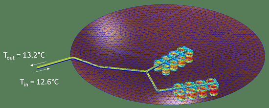
The closed-loop solution. 10 kW is extracted at this operating point. Note how the water heats up and cools down within the pond under these operation conditions.
Closing Remarks
You can see from the techniques we’ve outlined here that you can not only take an integral, but even solve for the limits of that integration, and make this equation a part of the rest of your model. The example presented here considers a heat exchanger. Where else do you think you could use this powerful technique?


Comments (1)
Yaohui Chen
May 14, 2014It is interesting.
In earlier versions, I have tried to incorporate some spatial integral operators directly into equations.
I had some impression that this makes the equation extremely heavy. And for some reason, I observe that the integral operation tends to use only one CPU core and leave others idle. Maybe it has been improved since.