

A lot of materials have anisotropic properties and, in many cases, the anisotropy follows the shape of the material. The COMSOL Multiphysics® software offers different methods for defining curvilinear coordinate systems. Here, we discuss the concepts of each and when to use which method.
Anisotropic Properties
Anisotropic properties are found in a wide variety of areas, such as rock formations with anisotropic seismic properties; liquid crystals used in LCD displays; materials for the aerospace industry, which must be lightweight and still withstand high loads; or soft tissues that biomedical replacements should mimic for optimal performance.
The Basics of Curvilinear Systems
In a previous blog post, we saw how to use the Curvilinear Coordinates interface and how to apply it to account for anisotropic thermal conductivity.
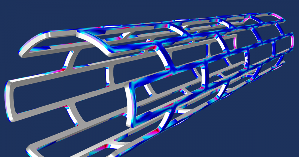
Let’s revisit this application and consider a carbon-fiber-reinforced polymer. The woven fibers embedded in an epoxy matrix have high thermal conductivity along the fiber axis and low conductivity in the cross section. It is almost impossible to express the anisotropy referring to the well-known Cartesian coordinate system. If we had a coordinate system that follows the fibers, it would be straightforward to specify the anisotropic properties.
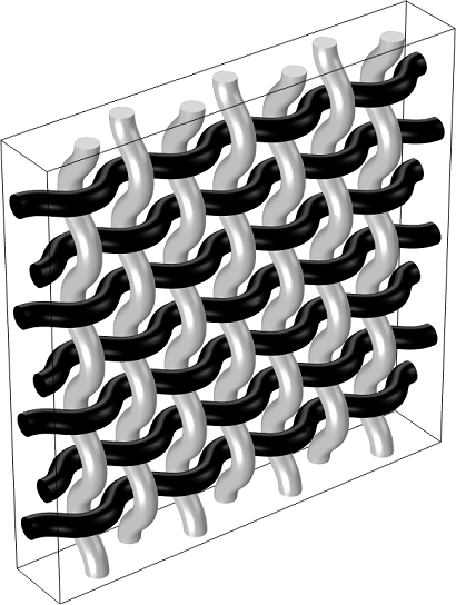
Woven fibers in an epoxy matrix.
How can such a coordinate system be determined? Physically, there are numerous effects that result in a vector field following the shape of the geometry; for instance, flow through the fibers or heat conduction from one end to the other or even a bundle of current-carrying wires that produce a magnetic field. These are precisely the methods that are used in the COMSOL® software to compute the curvilinear system. All methods compute a vector field, \mathbf{v}, which forms the first basis vector. Since most applications require a normalized vector field, COMSOL Multiphysics automatically normalizes by dividing with |\mathbf{v}|. A second vector field is specified manually, and one of the Cartesian coordinates is often a good choice. Starting from this, the second basis vector \mathbf{e}_2 is reconstructed to ensure that it is perpendicular to \mathbf{e}_1 and normalized. The cross product of these two gives the third base vector, \mathbf{e}_3.
Internally, the software uses the Cartesian coordinate system (\mathbf{e}_x,\ \mathbf{e}_y,\ \mathbf{e}_z) for computation and converts all quantities referring to a different coordinate system (\mathbf{e}_1,\ \mathbf{e}_2,\ \mathbf{e}_3). A direction given by a vector, \mathbf{F}=(F_1,\ F_2,\ F_3), in an arbitrary coordinate system can always be transformed into Cartesian coordinates, as follows:
e_{11} & e_{12} & e_{13} \\
e_{21} & e_{22} & e_{23} \\
e_{31} & e_{32} & e_{33}
\end{matrix}\right)\cdot\left(\begin{matrix} F_1\\F_2\\F_3\end{matrix}\right)=\mathbf{M}\left(\begin{matrix} F_1\\F_2\\F_3\end{matrix}\right)
Here, \mathbf{M} is the transformation matrix. For the inverse transformation, simply use the inverse, \mathbf{M}^{-1}, and if (\mathbf{e}_1,\ \mathbf{e}_2,\ \mathbf{e}_3) is orthonormal then \mathbf{M}^{-1}=\mathbf{M}^{T}.
Next, I will illustrate the different methods available in COMSOL Multiphysics that can be used to calculate a curvilinear coordinate system, which include the:
- Diffusion method
- Adaptive method
- Flow method
- Elasticity method
Let’s pick a single fiber and have a closer look.
Diffusion Method
The diffusion method solves Laplace’s equation: -\Delta U=0. The solution, U, is a scalar potential, and its gradient forms the first base vector. Because you solve for a single scalar potential only, this method is computationally inexpensive. The direction of the vector field is specified with the inlet and outlet boundary conditions. If the geometry is a closed loop, you can set the Jump boundary condition on an interior boundary to specify the direction.
The diffusion method is equivalent to solving the stationary heat conduction equation with constant temperatures at the inlet and outlet boundaries. The temperature gradient then forms the first base vector, as illustrated below.
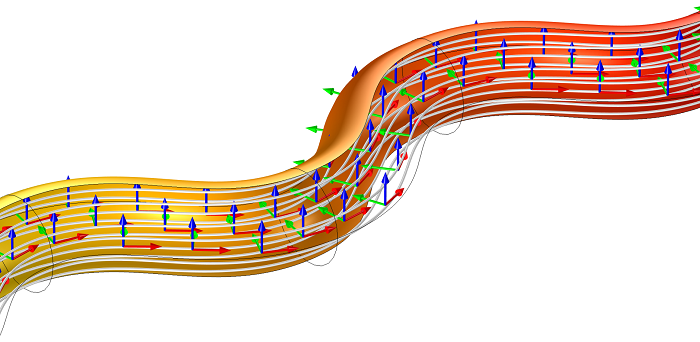
Curvilinear coordinate system (arrows), temperature gradient (streamlines), and temperature (surface).
Adaptive Method
The adaptive method, which is similar to the diffusion method, is based on Laplace’s equation as well. In addition, the resulting vector field is adapted to the shape of the geometry such that the streamline density is constant across the cross section of the geometry. This formulation is used to model multiturn coils (bundles of wires) in 3D magnetic applications with the AC/DC Module, an add-on to COMSOL Multiphysics. For multiturn coils, the current density should be roughly constant in the cross section, since it is assumed that each wire carries the same current and the wires are evenly spaced.
Flow Method
Here, you solve the incompressible Stokes equation for a vector field and a scalar. Thus, this method is the most computationally expensive. The boundary conditions are the same as for the diffusion method. A physical analogy would be incompressible creeping flow with a constant normal velocity at the inlet and a fixed pressure at the outlet. The resulting velocity field gives you the first base vector.
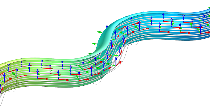
Curvilinear coordinate system (arrows), velocity field (streamlines), and pressure (surface).
Elasticity Method
The elasticity method solves the following eigenvalue equation:
where \mathbf{e} is the vector field, \mathbf{I} the identity matrix, and \lambdathe eigenvalue.
This method is slightly cheaper in terms of computational costs compared to the flow method because you solve for a vector field only. This difference in performance is more apparent in 2D models. The inlet and outlet boundary conditions are identical, \mathbf{e}\times \mathbf{n}=0. Prior to the implementation of the adaptive method, this method was used for modeling multiturn coils because it provided the best results in terms of constant streamline density in cross section.
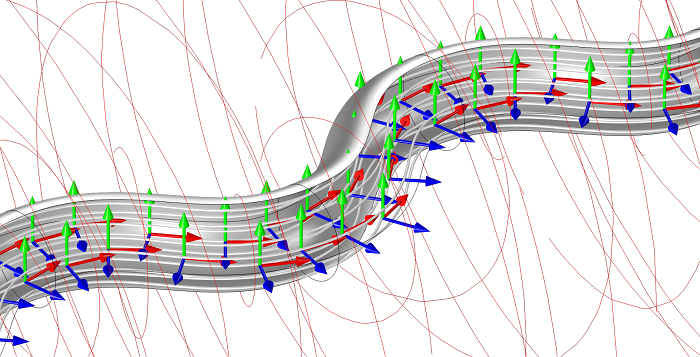
Curvilinear coordinate system (arrows), coil direction (gray streamlines) and magnetic flux density (red streamlines).
Apart from these predefined methods, the COMSOL® software also provides a user-defined input, as usual. You may encounter other scenarios where you want to implement curvilinear coordinates manually, such as anisotropic hyperelastic material for modeling collagenous soft tissue in arterial walls.
Which Method Should I Choose?
At first glance, all of the methods lead to the same coordinate system. However, some shapes require special attention, and the choice of the method can lead to significantly different results when the coordinate system is used for a physical application. Pay attention to geometries that have at least one of the following characteristics.
Curvature
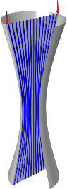
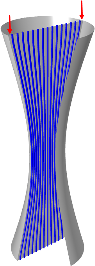
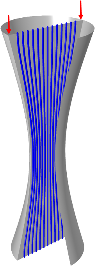
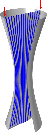
Let’s take a closer look at the streamlines for the various methods. Remember, the streamlines follow the vector field, which defines the first base vector. They start from equidistant points but follow different paths, as can be seen below.
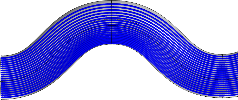 Diffusion method: Streamlines follow the “shortest” path.
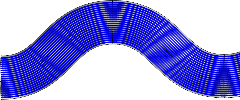 Adaptive method: Evenly distributed streamlines.
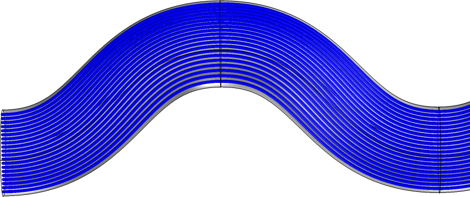 Elasticity method: Streamlines tend to accumulate at the convex bend.
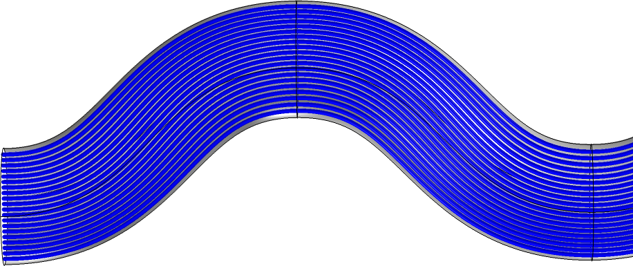 Flow method: Streamlines tend to accumulate at the convex bend.
If bends are very sharp, the characteristics of each method are more distinctive, and also the adaptive method can develop nonuniform streamline density.
Variable Cross Section
In this case, the elasticity method can fail, and you obtain an eigenvalue with eigenvectors that do not produce the required coordinate system. Alternatively, you may have to manually search for the correct eigenvalue. We can see that the streamlines also do not follow the shape perfectly at the upper part of the geometry. Similar, but not as distinctive, behavior is observed with the diffusion and adaptive methods. The flow method provides the best results here but is also the most computationally expensive.
 Diffusion method.
 Adaptive method.
 Elasticity method.
 Flow method.
Streamlines along the center plane of the geometry.
Application to Heat Transfer
Let’s go back to our model with the fibers that have an anisotropic thermal conductivity of 60\ W/mK in the fiber direction and 4\ W/mK perpendicular to this. If these directions coincide with the axes of the coordinate system, the thermal conductivity — a second-order tensor — has 0 off-diagonal elements.
k_{xx} & k_{xy} & k_{xz} \\
k_{yx} & k_{yy} & k_{yz} \\
k_{zx} & k_{zy} & k_{zz}
\end{matrix}\right)=\left(\begin{matrix}
60 & 0 & 0 \\
0 & 4 & 0 \\
0 & 0 & 4
\end{matrix}\right)
To be able to use this diagonal form, the curvilinear coordinate system for the fibers must be calculated prior to solving for the heat transfer. Because the geometry doesn’t have sharp bends or a changing cross section, the diffusion method gives a fast solution for the curvilinear coordinate system.
After that, you can refer to this coordinate system in the Heat Transfer in Fibers node. The anisotropy of the thermal conductivity can be defined in the Materials node, with the syntax k=\{60, 4, 4\}. Alternatively, you can select the user-defined input in the associated heat transfer node.
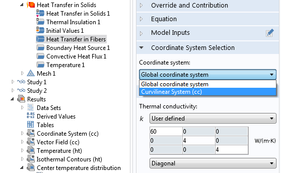
Definition of anisotropy in the associated heat transfer node.
In the model, a boundary heat source in the form of a Gaussian pulse is applied to the center of the geometry and the temperature spreads along the fibers.
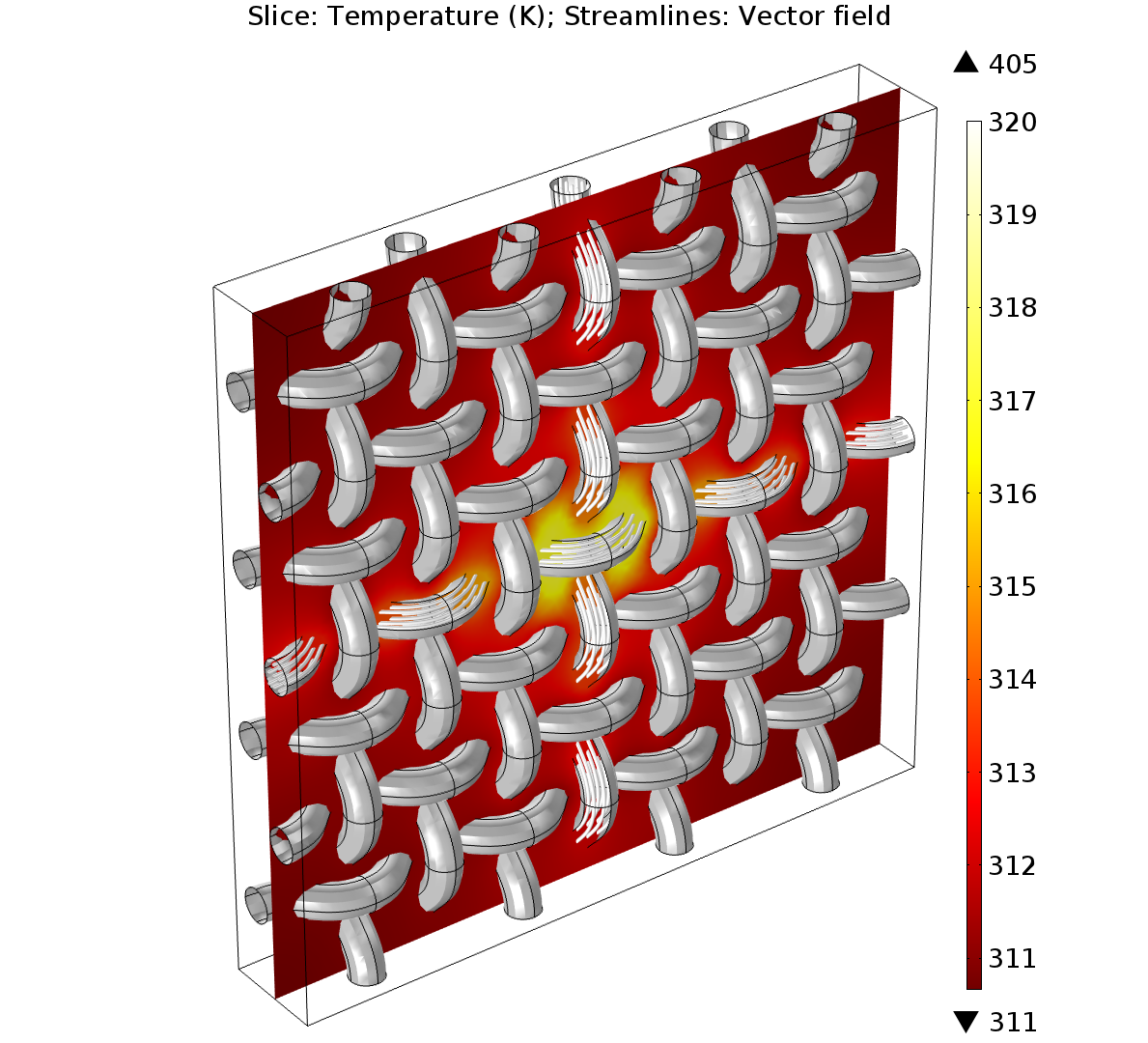
Streamlines indicate the vector field obtained with the Curvilinear Coordinates interface.
If you want to visualize, for example, the xx-component of the thermal conductivity (k_{xx}), keep in mind that you plot the xx-component in Cartesian coordinates (\mathbf{e}_x,\ \mathbf{e}_y,\ \mathbf{e}_z). Then, the thermal conductivity tensor, k, for the fibers is of nondiagonal form, according to the transformation described above. The local base vector system (\mathbf{e}_1,\ \mathbf{e}_2,\ \mathbf{e}_3), which was used to define k, is now varying through space and so does k_{xx}. In this model, you can plot the components of the thermal conductivity vector in a Slice plot, for example. You can select them from the Expressions menu in the corresponding Settings window or simply type ht.kxx (where ht is the tag for the Heat Transfer in Solids interface that was used for this model).
Concluding Remarks
This blog post has described the different methods for defining the curvilinear coordinate systems that are available in COMSOL Multiphysics as well as when to choose one over another.
In summary, the adaptive method provides the best solution for most cases at comparatively low computational costs. The diffusion method has even lower computational costs and is suitable for simple geometries without bends or varying cross sections. The other methods can be advantageous in some cases and are interesting for certain applications.
- Diffusion method
- Pros: low computational cost
- Cons: computed vector field tends to take the shortest path in bends
- Adaptive method
- Pros: low computational cost, provides the best solution for most cases
- Cons: variable cross sections not always handled perfectly
- Elasticity method
- Pros: computational cost lower than the flow method, better representation of moderate bends than diffusion method
- Cons: often requires manual selection of the eigenvalue and is not robust in all cases
- Flow method
- Pros: robust method, supports cross-section changes and sharp bends
- Cons: computational cost is often greater
To try the carbon fiber model presented here, click the button below.
Editor’s note: This blog post was updated on December 5, 2018, to include information on the adaptive method.

Comments (11)
Ivar Kjelberg
February 17, 2015Hi Nancy
Thanks for å detailed discussion, I have one issue though:
I need to consider aniso-tropic thermal expansion, but I have no coordinate frame selection list to choose from in the thermal expansion sub-node, in contrary to your example of the thermal conduction k.
So what are the correct equations & variable names to use in this case? V5.0
Sincerely
Ivar
Yangguang Ou
December 16, 2015Thank you for the helpful blog!
Numi Rumi
October 10, 2017Can we use curvilinear coordinates for time domain study?
Nancy Bannach
October 10, 2017Dear Numi,
there should be no problem when you first solve the Curvilinear Coordinates (stationary) to get your coordinate system and then use this in a time dependent study for heat transfer, for example.
A time changing coordinate system is not possible, as far as I know. If you are interested in something like this I recommend to discuss this with our support team in more detail via https://www.comsol.com/support
Best Regards,
Nancy
Mst Nazmunnahar
February 14, 2018Hi,
Thanks for this helpful blog. Can we use this anisotropic thermal conductivity under Heat transfer in solid(ht) sub-node solid 1 node or we need to add another node? Which node we should add for anisotropic thermal conductivity?
Thanks
Nancy Bannach
February 15, 2018Dear Mst Nazmunnahar,
you can also use it for solid, of course. Whenever you have the settings as shown in the image with the caption “Definition of anisotropy in the Heat Transfer node.”: An option to select a coordinate system and the option to define anisotropic material properties. So, you can use this approach in other physics as well.
Best regards,
Nancy
Anonymous
April 25, 2018Dear Nancy,
Hi! For me I applied creeping flow module with the porous media domains on, and I can only define the permeability of the porous media in “Fluid and Matrix Properties” interface and there is no option to choose the coordinate system like you shown to define the material property based on defined Curvilinear Coordinates as presented in the attachment. Could you help me to find a solution for this problem? Thanks a lot!
Nancy Bannach
April 26, 2018Hi,
thanks for your feedback. You are right, there is no option to select another coordinate system for the Fluid and Matrix properties.
The only option I see at the moment is, that you define the components manually. You can have a look at the model carbon_fibers.mph (https://www.comsol.com/model/anisotropic-heat-transfer-through-woven-carbon-fibers-16709).
The definition of each component is written in the Equation View below the “Solid 2” node. You can adapt this definition for your problem.
If you need further assistance, please contact our Technichal Support team https://www.comsol.com/support.
In the meantime, I will forward this to our developers.
Best regards,
Nancy
Sergey Kuznetsov
September 12, 2018Hello!
I was wondering where I can find the detailed comments in the creating Woven Carbon Fibers Geometry.
The pdf document https://www.comsol.com/model/download/449671/models.heat.carbon_fibers_geom.pdf
says that instructions are in the “Anisotropic Heat Transfer through Woven Carbon Fibers.”
But the that document (https://www.comsol.com/model/download/469631/models.heat.carbon_fibers_infinite_elements.pdf) doesn’t have steps on creating geometry, instead it offers to open existin geometry “carbon_fibers_geom.mph”.
Can i find anywhere actual instruction to create the geometry?
Thank you!
Nancy Bannach
September 13, 2018Dear Sergey,
you are right, there is no section on how to create the geometry. The sentence in the pdf file refers to the whole model set-up (not geometry set-up).
If you are interested in how to create geometries in general I recommend to have a look at our video gallery
https://www.comsol.com/videos?type%5B%5D=videotype-tutorial&workflow%5B%5D=workflowstep-geometry&s=
Otherwise you can always have a closer look at the Geometry node and every single node that is used to build the geometry. E.g. when you right-click on “Work Plane 1” in the geometry of the carbon fiber model you can choose “Build selected”. Then the geometry is build from the top node up to the Work Plane node.
You can expand the Work Plane node to see, what is done there. Then go to “Sweep” and do the same and so on.
I hope this helps. You can also contact our support team (https://www.comsol.com/support) in case you get stuck with your own geometry.
Best regards,
Nancy
Sergey Kuznetsov
September 15, 2018Dear Nancy, thank you for explaining this!