

Creating animations is an effective way to present and visualize simulation results. In COMSOL Multiphysics, this is fairly straightforward using the Player node for time-dependent or parameter sweep study types. But, can we animate how the solution changes along a direction in a 3D steady-state model? The answer is yes. Here, we will learn how to combine parallel slices to create an animation for a 3D steady-state example model, using a three-step process.
Animation for a 3D Steady-State Model
In a 3D model, we are often interested in understanding how a solution evolves along a particular direction. Let’s consider the 3D Laminar Static Mixer model, where the fluid velocity and concentration distribution are primarily varying along the axial direction. This model shows how the static geometric obstacles induce secondary flows in the device, which, in turn, improve the mixing characteristics. The plot below shows the steady-state concentration distribution on parallel sections (or slices).
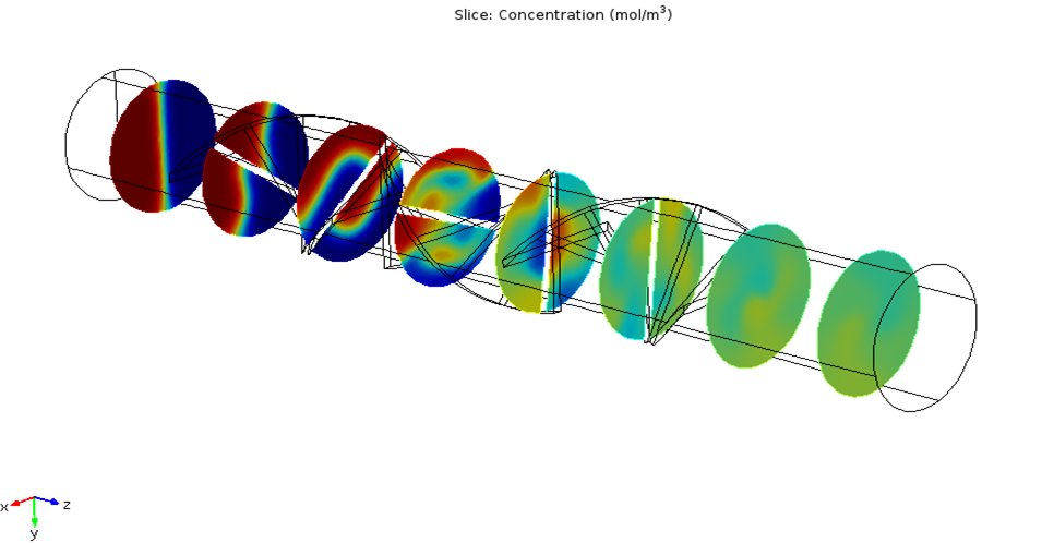
Concentration slice plot in a laminar static mixer.
The plot shows how the concentration changes from a perfectly unmixed state to a mixed state. Let’s look at how we can present this information using an animation. Our objective is to stitch the static slices together to create the frames of a movie.
Creating the Animation
Step 1
The first step is to add a parameter corresponding to the axial coordinate. For this example model, we add a parameter zp as shown in the screenshot below.
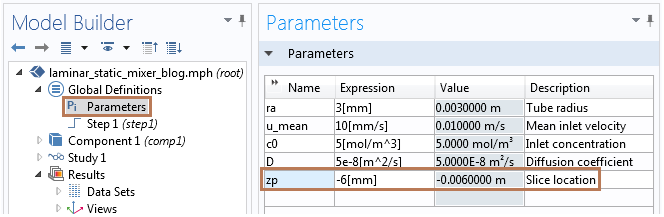
Adding a parameter in the Parameters table.
If you are using COMSOL Multiphysics® version 5.2a, then the parameter zp must be defined under the Results node. Right-click the Results node, select “Parameters”, and define zp as shown in the screenshot below.
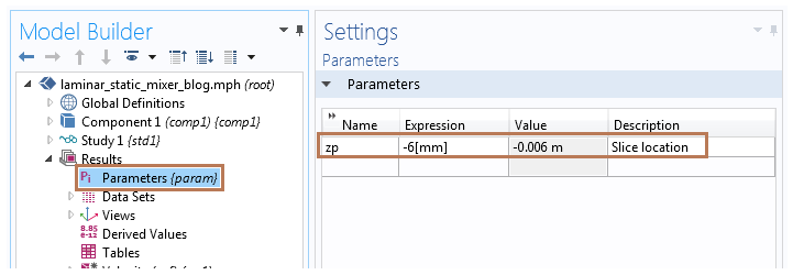
Editor’s note: This section of the blog post was updated on 12/14/2016 to reflect updates in COMSOL Multiphysics version 5.2a.
Step 2
Second, we need to change the slice plot settings. In the Plane Data section, let’s change the Entry Method to “Coordinates” with zp as the input to the z-coordinates field. These changes enable us to plot the solution in the plane z = zp.
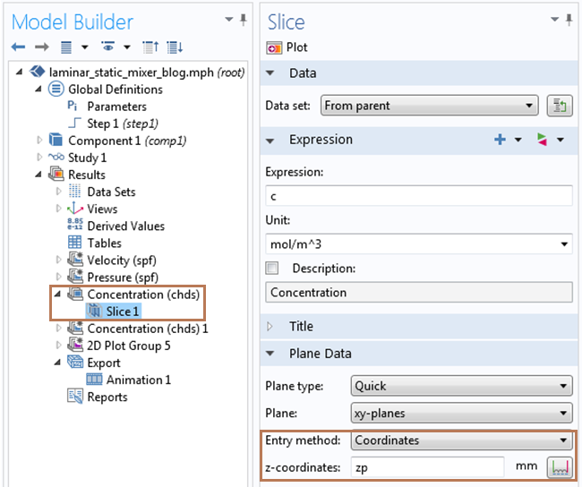
Plane data settings for concentration slice plot.
Step 3
Last, we need to add an Animation or Player node to the model (right-click on Export under the Results node and choose “Animation”). We would like to generate an animation that plots the solution as the slice location zp moves from one end of the mixer to the other.
In the Animation settings, choose the Subject as “Concentration (chds)”, which is the concentration slice plot.
Now, let’s change the Sequence type to “Result parameter” with zp as the Parameter ranging from -6 to 36, as shown below. One could also use similar animation settings in the Player node (right-click on Export and choose “Player”) to visualize animations within the COMSOL Desktop.
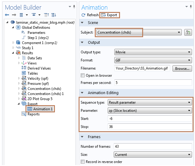
Animation settings for changing the slice location.
Now, click on the Export button to create the desired animation. The resulting animation for our Laminar Static Mixer model appears below.
Animation showing concentration evolution along the axial direction.
It is simple to further customize your animations in terms of frame rate, orientation, animation format, etc. This is done through various options in the Animation and Plot settings. For example, the following animation shows the same animation with an xy view without the data set (geometric) edges.
Animation showing concentration evolution (xy view) along the axial direction without the data set edges.
Summary
We have used a very simple three-step procedure to combine cross-sectional data (parallel slices) to create an animation for a 3D steady-state model. Now, suppose we are interested in finding the maximum (or minimum) value of any variable in each of these parallel slices.
Do you think we can create a plot of cross-sectional maximum (or minimum) values along the axial direction? I will address this post-processing question in a follow up blog entry. Stay tuned!

Comments (4)
Ivar Kjelberg
August 27, 2014Thank you Mranal for this interesting and useful trick / feature 🙂
Jeff Stevens
November 8, 2016If you are using COMSOL 5.2a, the above method won’t work.
Per COMSOL support, here is what you should do:
“Because of the update in the software, this parameter now needs to be
created under the Results node. You can do this by right-clicking the
Results node and choosing the Parameters option. Once you define the zp parameter in the Result>Parameters node, this variable is available for use in the Animation node. “
Mranal Jain
November 9, 2016Thanks Jeff. We are in the process of updating this blog to reflect the new settings in the latest version.
Mohammad Amin Kazemi
February 17, 2017Thank you for this post. I really loved it.