

Buckling instability is a treacherous phenomenon in structural engineering, where a small increase in the load can lead to a sudden catastrophic failure. In this blog post, we will investigate some classes of buckling problems and how they can be analyzed.
What Is Buckling?
Have you ever seen the party trick where a full-grown person can balance on an emptied soda can?
Even though the can’s wall is only 0.1 millimeter thick aluminum, it can sustain the load as long as its shape is perfectly cylindrical. The axial stress is below the yield stress, which is easily checked by just dividing the force by the cross section area.
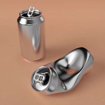
But, if you just press lightly against a point on the cylindrical surface, the can will collapse. The collapse load for the perfect cylinder is higher than the weight of the person performing the trick, while only a slight distortion will significantly decrease the load bearing capacity. This phenomenon is called imperfection sensitivity and is one of the possible pitfalls when designing structures under compression. You can see some cases of collapsed shells with dimensions much larger than soda cans on this page.
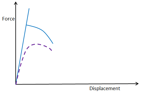
Mathematically, buckling is a bifurcation problem. At a certain load level, there is more than one solution. The sketch below shows a bifurcation point and three different possible paths for the solution, branching out at the bifurcation point. The secondary path can be of three fundamentally different types as indicated in the sketch.
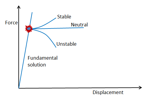
A solution with a bifurcation.
If the load carrying capacity continues to increase, the solution can be characterized as stable. This is the least dangerous situation, but if you fail to recognize it, you will probably compute too low stresses. Thereby you will underestimate the load carrying capacity. The neutral and unstable paths are more dangerous, since once the peak load is reached, there is no limitation of the displacements.
When there is more than one solution, the question about which one is correct arises. All solutions will satisfy the equations of equilibrium, but in real life, the structure will have to select a path. It will do so based on where the energy can be minimized. The solution you compute using conventional linear theory will in general not be the preferred solution.
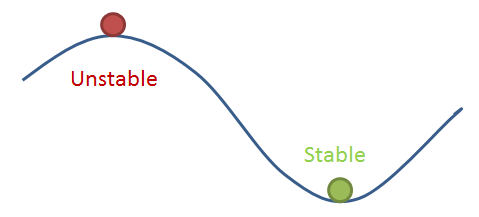
You can make the analogy with a ball on a wavy surface. It can be in equilibrium both on the hilltops and in the valleys, but any perturbation will make it drop into the valley. In the same way, even the smallest perturbation to the structure will make it jump to the more energetically preferable state. In real life, there are no perfect structures; there will always be perturbations in geometry, material, or loads.
Linearized Buckling Analysis
The easiest way in which you can approach a buckling problem is by doing a linearized buckling analysis. This is essentially what you do with pen and paper for simple structures in basic engineering courses. Computing the critical loads for compressed struts (like the Euler buckling cases) is one such example.
In COMSOL Multiphysics, there is a special study type called “Linear Buckling”. When performing such a study, you add the external loads with an arbitrary scale. It can be a unit load or the intended operating load. The study consists of two study steps:
- A Stationary study step where the stress state from the applied load is computed.
- A Linear Buckling study step. This is an eigenvalue solution where the stress state is used for determining the Critical load factor.
The critical load factor is the factor by which you need to multiply the applied loads to reach the buckling load. If you modeled with operational loads, the critical load factor can be interpreted as a factor of safety. The critical load factor can be smaller than unity, in which case the critical load is smaller than the one you applied. This in itself is not a problem, since the analysis is linear. The critical load factor can even be negative, in which case the lowest load needed for buckling acts in the opposite direction from the one in which you applied the load.
The eigenvalue solution will also give you the shape of the buckling mode. Note that the mode shape is only known to within an arbitrary scale factor, just like an eigenmode in an eigenfrequency analysis.
Before going into detail, some words of warning are appropriate:
- For some real-life structures, the theoretical buckling load obtained using this approach can be significantly higher than what would be encountered in practice due to imperfection sensitivity. This is especially important for thin shells.
- Some structures show significant nonlinearity even before buckling. The reasons can be both geometrical and material nonlinearity.
- Never use symmetry conditions in a buckling analysis. Even though the structure and loads are symmetric, the buckling shape may not be.
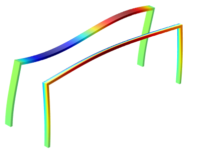
The buckling shapes of two symmetric frames with slightly different cross sections and equal symmetric load.
The idea with the linearized buckling analysis is that the problem can be solved as a linear eigenvalue problem. The buckling criterion is that the stiffness matrix is singular, so that the displacements are indeterminate. The applied set of loads is called \mathbf P_0, and the critical load state is called \mathbf P_c = \lambda \mathbf P_0, where \lambda is a scalar multiplier.
The total stiffness matrix for the full geometrically nonlinear problem, \mathbf K, can be seen as a sum of two contributions. One is the ordinary stiffness matrix for a linear problem, \mathbf K_L, and the second is a nonlinear addition, \mathbf K_{NL}, which depends on the load.
In the linear approximation, \mathbf K_{NL} is proportional to the load, so that
The stiffness matrix is singular when its determinant is zero. This forms an eigenvalue problem for the parameter, \lambda.
The lowest eigenvalue \lambda is the critical load factor, and the corresponding eigenmode, \mathbf u, shows the buckling shape.
By default, only one buckling mode corresponding to the lowest critical load is computed. You can select to compute any number of modes, and for a complex structure this can have some interest. There may be several buckling modes with similar critical load factors. The lowest one may not correspond with the most critical one in real life due to, for example, imperfection sensitivity.
In the COMSOL software, you should not mark the Linear Buckling study step as being geometrically nonlinear. The nonlinear terms giving \mathbf K_{NL} are added separately. However, if you do select geometric nonlinearity, you will solve the following problem:
The the extra ‘1’ in the term\lambda+1 is automatically compensated for, so the computed load factor is the same in either case. The best rule is to use the same setting for geometric nonlinearity in both the preload study step and the buckling study step.
You can study an example of a linearized buckling analysis in the model Linear Buckling Analysis of a Truss Tower.
Fixed Loads and Variable Loads
Sometimes, there is one set of loads, \mathbf Q, which can be considered as fixed with respect to the buckling analysis, whereas another set of loads, \mathbf P_0, will be multiplied by the load factor \lambda. Still, the combination of both load systems must be taken into account when computing the critical load factor.
Mathematically, this problem can be stated as
This kind of problem can also be solved in COMSOL Multiphysics using one of two strategies:
- Run it as a post-buckling analysis, with one set of loads fixed and the other set of loads ramped up. This is straightforward, but unnecessarily heavy from the computational point of view.
- Use a modified version of the Linear Buckling study as described below.
Due to the flexibility of the software, it is not difficult to modify the built-in Linear Buckling study so that it can handle the two separate load systems. To do that, start by adding an extra physics interface, which is used only to compute the stress state caused by the fixed load. Solve for this interface only in the stationary analysis, but not in the buckling step.
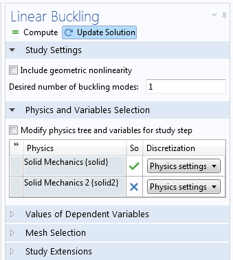
The extra physics interface is not active in the Linear Buckling step.
Now, you need to generate the extra stiffness matrix contribution in the buckling study from the stresses that were computed in the second physics interface. You do that by adding the following extra weak contribution:
Here, \boldsymbol \sigma^{Q} is the stress tensor from the fixed load, and \mathbf E and \boldsymbol \epsilon are the Green-Lagrange and linear strain tensors, respectively. In other words, the difference \mathbf E-\boldsymbol \epsilon contains the quadratic terms of the Green-Lagrange strain tensor.
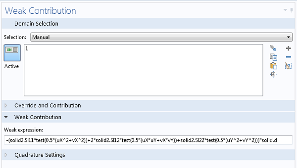
Contribution from the fixed load system for a 2D Solid Mechanics problem.
Now, you can run the study sequence as usual, and the computed critical load factor applies only to the second load system.
Post-Buckling Analysis
With a linearized buckling analysis, you will only find the critical load, but not what happens once it has been reached. In many cases, you are only interested in ensuring the safety against reaching the buckling load, and then a linearized study may be sufficient.
Sometimes, you will, however, need the full deformation history. Some of the reasons for this might be:
- The structure has significant nonlinearity also before the critical load, so a linearized analysis is not applicable.
- You need to investigate imperfection sensitivity.
- The operation of the component intentionally acts in the post-buckling regime.
In order to perform a post-buckling analysis, you will need to load the structure incrementally, and trace the load-deflection history. In the COMSOL software, you can use the parametric continuation solver to do this.
Doing a post-buckling analysis is not a trivial task. An inherent problem is that there are several solutions to a bifurcation problem, so how do you know that the solution you get is as intended? Also, in many cases the buckling instability will manifest itself numerically as an ill-conditioned or singular stiffness matrix, so that the solver will fail to converge unless you use appropriate modeling techniques. Below, I outline some useful approaches.
Symmetric Structures
Consider a simple case like a cantilever beam with a compressive load at the tip. When it reaches the collapse load, it can deflect in an arbitrary direction in 3D, or in two possible directions in 2D. It is, however, unlikely that the solver will converge to any of these solutions, unless the symmetry is disturbed since the symmetric problem will become singular at the buckling load. If you add a small transverse load at the tip, the solution can be traced without problems. An example using this technique can be found in the Large Deformation Beam model.
Snap-Through Problems
In many cases, the structure will “jump” from one state to another. A simple example of this can be displayed by the two-bar truss structure below.
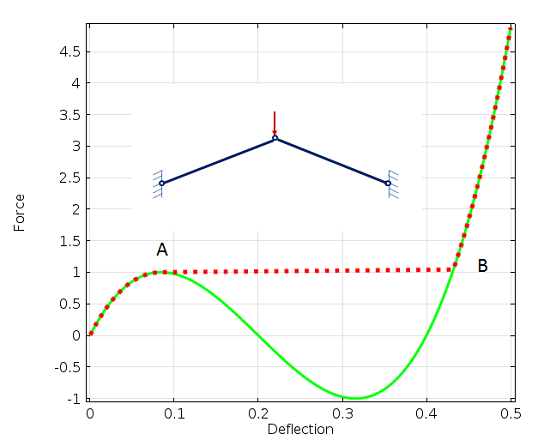
Snap-through analysis of a simple truss structure. At deflection 0.2, the two bars are horizontal.
When the force is increased, it will reach the peak value at A. Numerically, the stiffness matrix will become singular. Physically, the structure will suddenly invert and jump to the state B along the red dotted line. In real life, this will be a dynamic event. The stored strain energy will be released and converted into kinetic energy.
One way of solving this problem is to actually run a time-dependent analysis, where the inertia forces will balance the external load and internal elastic forces. However, such an approach is seldom used, since it is computationally expensive.
To trace the solid green line, you can replace the prescribed load by a prescribed displacement, and instead record the reaction force. Replacing loads with prescribed displacements is a simple method to stabilize models, but the method has limitations:
- It is more or less limited to cases where the external load is a single point load.
- The displacement you prescribe must be monotonically increasing.
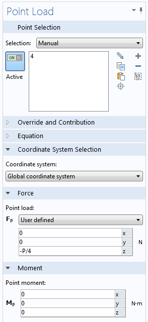
To introduce a more general method, consider the shallow cylindrical shell below. It is subjected to a single point load at the center, so in this case it would also be tempting to use displacement control. But, as you can see in the graph below, neither the force nor the displacement under the force is monotonic during the buckling event.
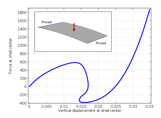
A shallow cylindrical shell and graph of the load versus displacement.
Animation of the buckling event.
For problems like this, literature will recommend that you use an arc-length solver. The popular Riks method is one such method, and we are frequently asked why we do not add such a solver to our software. The simple answer is that we do not need one.
A problem like this one is actually quite easy to solve using the continuation solver in COMSOL Multiphysics, once you have learned how to do it. All you need is to figure out a quantity in your model that will increase monotonically, and then use it to drive the analysis. For instance, in the model above, you can select the average vertical displacement of the shell surface as the controlling parameter.
You will then add the load intensity as an extra degree of freedom in the problem, introduced through a Global Equation. The equation to be fulfilled is that the average displacement (defined through an average operator) should be equal to the continuation parameter (called disp in the screenshot below).
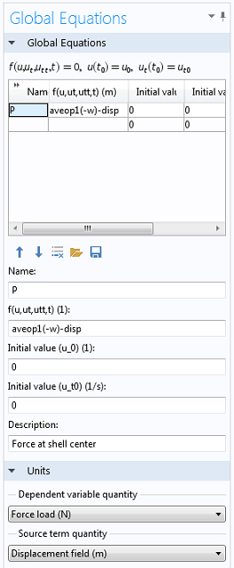
Adding a Global Equation to control the load.
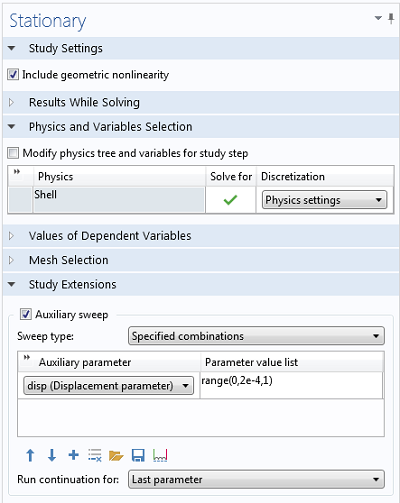
The Stationary solver is set up to run the continuation sweep.
You can download the full model from the Model Gallery.
The method I just described above is by no means limited to buckling problems in mechanics. It can be used for any unstable problem, like a pull-in analysis of an electromechanical system, for example.
Imperfections
Occasionally, it is necessary to model imperfections explicitly. As an example, there are standards stating that a load must have a certain eccentricity, or that a beam must have a certain assumed initial curvature. When you introduce an imperfection, the load-deflection curve will take a “shortcut” between the branches of the ideal bifurcation curve.
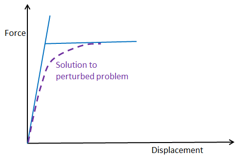
Solution path for a model with initial imperfection.
When you include a disturbance in the model of a geometry that is imperfection sensitive, the peak load may decrease significantly. This is what happens to the soda can in the scenario mentioned earlier, and it is a physical reality, not just an effect of finite element modeling. Thus, it is of the utmost importance to actually take imperfections into account for this class of structures.
Solution path for a model with imperfection sensitivity.
How should you then select an appropriate imperfection in your model?
One good strategy is to first perform a linearized buckling analysis and then use the computed mode shape as imperfection. The idea is that the structure will be most sensitive to this shape. It is, however, not essential that you capture the exact shape, so you could use anything similar. The size of the perturbation should be similar to what you would expect in your real structure when considering manufacturing tolerances and operating conditions.
In some cases, it also a good idea to compute several buckling modes and try more than one of them if the critical load factors are of the same order of magnitude. The imperfection sensitivity can vary a lot between different buckling modes.
Instead of actually changing the geometry, it is often easier to obtain the perturbation using an additional load. If you do so, you should make sure that the stresses introduced by that load do not significantly change the problem.
Further Reading
- Overview of buckling
- Information on buckling of shells
- Explore the software:

Comments (14)
Ivar Kjelberg
March 10, 2014Hi Henrik
Thanks for a detailed explanation and some nice tricks, the one with combined static and buckling loads is of high interest, I had though of something like that but hadn’t dare try it to now, but I’ll check it next time I need a buckling analysis, as for me it applies to most of my buckling cases. (PS what about typing out in text the corrected formula for 3D, as we cannot “Cut&Paste from the bitmap image 😉
I always complete my buckling modal analysis by non-linear analysis, even if these can take a few hours (or days) when the solver starts to loop around. In fact, often the true non-linear geometry part is only a small fraction of my model volume, (but often half the mesh number) so it could be nice to be able to split the task to lower the non-linear DOFs. Any suggestions how to reduce the model complexity.
Rigid domains is one way, but with complex geometries it still uses many mesh DOFs
What I notice is that if one only rely on single beam buckling analysis, and try to apply that to complex “compliant (flexing) structures”, one fails, as many of the buckling modes are suppressed by the full 3D geometry layout, and in some loaded cases one can get the 3rd or 5th mode only that accepts to buckle, hence a safety factor 2-4 times higher than thought. As well as cases where the catastrophic buckling (when the supporting force tends to zero after the buckling knee) might transform to a constant force solution, which is often sufficient for a structure to survive.
But I can only stress, the importance of testing, as FEM is just a model of reality and models are to be admired, not really to trust, alone …
Sincerely
Ivar
Henrik Sönnerlind
March 14, 2014Thanks for the comments, Ivar.
Here are the expressions you asked for, ready for Copy-Paste.
Solid 3D:
-(solid2.SX*test(0.5*(uX^2+vX^2+wX^2))+2*solid2.SXY*test(0.5*(uX*uY+vX*vY+wX*wY))+2*solid2.SXZ*test(0.5*(uX*uZ+vX*vZ+wX*wZ))+solid2.SY*test(0.5*(uY^2+vY^2+wY^2))+2*solid2.SYZ*test(0.5*(uY*uZ+vY*vZ+wY*wZ))+solid2.SZ*test(0.5*(uZ^2+vZ^2+wZ^2)))
Solid 2D:
-(solid2.SX*test(0.5*(uX^2+vX^2))+2*solid2.SXY*test(0.5*(uX*uY+vX*vY))+solid2.SY*test(0.5*(uY^2+vY^2)))*solid.d
Henrik
Benedikt Weber
August 26, 2014Hi Hendrik
Thanks for the overview of different ways to treat the buckling problem. I have done a linear static analysis followed by a linear buckling analysis. How would I proceed to use the buckling shape as an initial imperfection for a geometrically nonlinear analysis? I can use the buckling solution as initial value, but it has to be scaled, since the buckling shape has an arbitrary magnitude. However, I could not find a way to do this.
Benedikt
Henrik Sönnerlind
August 26, 2014Henrik Sönnerlind
August 26, 2014Hi Benedikt,
I will outline a procedure below (assuming that a 2D Solid Mechanics interface is used):
1. Run the buckling analysis in the Solid Mechanics with the default displacement degrees of freedom (u,v)
2. Check the maximum displacement of the arbitrarily scaled mode. Lets assume that you think that 1/400 of that value would form a good imperfection.
3. Add a Deformed Geometry interface.
4. Add a Prescribed Mesh Displacement (domain level). Select all domains, and enter ‘u/400’ and ‘v/400’ as the displacements.
5. Add another Solid Mechanics interface. As a default it has degrees of freedom (u2,v2).
6. Use the same boundary conditions as in the linearized buckling study. Enter the load as depending on some parameter ‘para’.
7. Add a Stationary study, and select ‘Geometric nonlinearity’.
8. Deselect the first Solid Mechanics interface in the new study so that only the two new interfaces are solved for.
9. Select ‘Variables not solved for’ and choose to take data from Study 1.
10 Select ‘Auxiliary sweep’ and enter an appropriate range for the load parameter.
Regards,
Henrik
壹 王
June 5, 2020Hi, Dr. Henrik Sönnerlind:
The method you provided for solving post-buckling problem has given me a great help. I am solving a post-buckling problem of a beam using the procedure you gave. However, I can’t select the beam in the “Prescribed Mesh Displacement” module. If possible, can you please give me some suggestions?
Regards,
Yi Wang
Henrik Sönnerlind
June 10, 2020 COMSOL EmployeeUnfortunately, your question does not contain enough details to be possible to answer. I suggest that you repeat it on the user forum, together with a model or some graphics that explain what you want to achieve.
Regards,
Henrik
Benedikt Weber
August 28, 2014This works well, but replicating the model can be error prone for more complicated cases. Also the deformed geometry is recalculated for each parameter in the sweep. Therefore I tried the following alternative. It needs an extra Study for calculating the deformed geometry but it uses only one Solid Mechanics interface and calculates the deformed geometry only once.
5. Add a Stationary study for calculating the deformed geometry, deselect the Solid Mechanics interface.
6. Select ‘Variables not solved for’ and choose to take data from Study 1.
7. Add a Stationary study, select ‘Geometric nonlinearity’ and deselect the Deformed Geometry interface
8. Select ‘Variables not solved for’ and choose to take data from Study 2.
9. Select ‘Auxiliary sweep’ and enter an appropriate range for the load parameter.
Regards,
Benedikt
Henrik Sönnerlind
September 1, 2014Hi Benedikt,
Your approach shows a very good solution.
Regards,
Henrik
Yu Zhang
June 28, 2018Hi, Dr. Henrik Sönnerlind:
It is really an interesting and useful approach to solve the softening problems. However, I am not sure it is applicable to my problem, i.e. time dependent fracturing processes caused by damage. I found it was not easy to apply your method to my case. Could you please provide me some ideas? Actually, I still want to solve my problems by arc-length method, but I am not sure whether I can achieve the method in COMSOL through Matlab or other programming tools. If possible, would you mind sharing me some ideas how to do that? Thank you for your help.
Yu
Henrik Sönnerlind
June 28, 2018Hi Yu,
Fracturing processes are particularly nasty, in that you may get a negative stiffness in many locations at the same time, as discussed in https://www.comsol.com/blogs/can-a-stiffness-be-negative. Also, there tends to be local breakdown in individual Gauss points, so regularization techniques are useful in order to smooth the damage.
Creating an arc-length solver of your own seems like a rather tough task; I have seen some attempts but more on buckling type problems where the number of instabilities are small.
An idea, just off the top of my head: Maybe you can try using (total) energy dissipation as your controlling variable in the method suggested in this blog post?
Also, giving a small random spatial variation of the material strength may help improving stability, since the locations for fracture initiation are better defined.
Regards,
Henrik
Yu Zhang
June 29, 2018Hi, Dr. Henrik Sönnerlind:
Thank you so much for your detailed reply and the valuable suggestions. As you mentioned, the energy dissipation may serve as a controlling variable to do the analysis like the approach you provided in this blog. Indeed, the energy dissipation (and also the damage variable) will monotonically increase in my problem. However, using these two variables to drive the simulation seems not as direct as using the average displacement to do so. In your approach, the average displacement can be applied as a boundary condition, but the energy dissipation and the damage, in my case, cannot be applied as a form of boundary condition. So, could you please share me some ideas to achieve that?
In addition, the problem in your blog is static. Is it also applicable to the time dependent problems?
Thank you so much for your help and time.
Best regards,
Yu
Peter Cendula
December 2, 2020Hi Henrik,
thank you for the excellent post.
I’m trying to use continuation solver for square thin shell buckling (thickness 100 nm, side length 140 micrometer) with initial compressive stress (load) and clamped perimeter of the square. I ramp the initial stress as monotonic parameter. In this way, Comsol computes post-buckling shape quite well and the shape loses reflection and rotation symmetry (as expected from experiment for large compressive stress). However, beyond some threshold stress, Comsol cannot solve it further – my hypothesis is that Comsol has difficulty to snap-through a different buckling shape. What would you suggest in order to enable convergence of the solution for even larger initial stress?
Sincerely
Peter
Xuecui Zou
November 28, 2021Hi Henrik,
I would like to ask if I would like to simulate the eigenfrequency of a buckled fixed-fixed beam, I used the displacement control the load on the center point of the beam, but the vibration mode I can get is only the second mode and the fourth mode, it missed the first mode. could you please give me any suggestions regarding to this?