
When a tuning fork is struck, and held against a tabletop, the peak frequency of the emitted sound doubles — a mysterious behavior that has left many people baffled. In this blog post, we explain the tuning fork mystery using simulation and provide some fun facts about tuning forks along the way.
Explaining the Tuning Fork Mystery
In a recent video on YouTube from standupmaths, science enthusiasts Matt Parker and Hugh Hunt discuss and demonstrate the “mystery” of a tuning fork. When you strike a tuning fork and hold it against a tabletop, it seems to double in frequency. As it turns out, the explanation behind this mystery can be boiled down to nonlinear solid mechanics.
How Does Sound Reach Our Ears?
When you hold a vibrating tuning fork in your hand, the bending motion of the prongs sets the air around them in motion. The pressure waves in the air propagate as sound. You can hear it, but it is not a very efficient conversion of the mechanical vibration into acoustic pressure.
When you hold the stem of the tuning fork to a table, an axial motion in the stem connects to the tabletop. The motion is much smaller than the transverse motion of the prongs, but it has the potential to set the large flat tabletop in motion — a surface that is a far better emitter of sound than the thin prongs of a tuning fork. The tabletop surface will act as a large loudspeaker diaphragm.
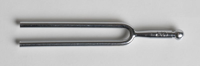
Our tuning fork.
To investigate this interesting behavior, we created a solid mechanics computational model of a tuning fork. The model is based on a tuning fork that one of my colleagues keeps in her handbag. The tone of the device is a reference A4 (440 Hz), the material is stainless steel, and the total length is about 12 cm.
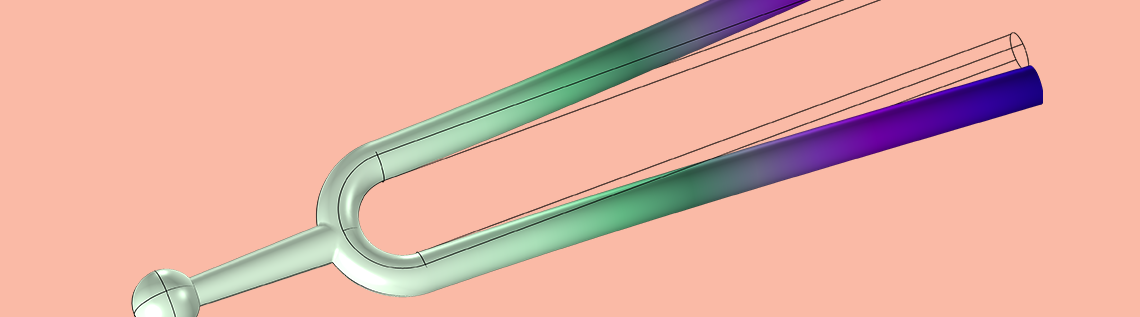
First, let’s have a look at the displacement as the tuning fork is vibrating in its first eigenmode:
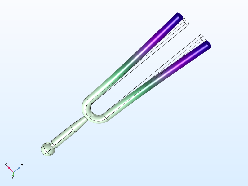
The mode shape for the fundamental frequency of the tuning fork.
If we study the displacements in detail, it turns out that even though the overall motion of the prongs is in the transverse direction (the x direction in the picture), there are also some small vertical components (in the z direction), consisting of two parts:
- The bending of the prongs is accompanied with an up-down motion that varies linearly over the prong cross section
- The stem has an essentially rigid axial motion, which is necessary for keeping the center of mass in a fixed position, as required by Newton’s second law
The displacements are shown in the figures below. The mode is normalized so that the maximum total displacement is 1. The peak axial displacement is 0.03 and the displacement in the stem is 0.01.
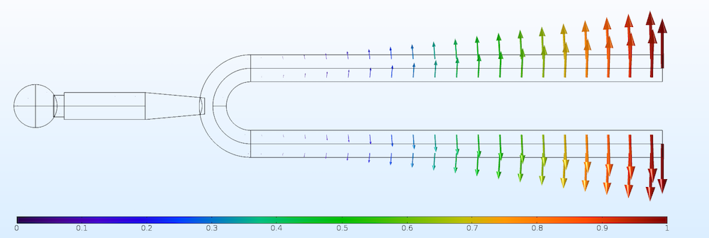
Total displacement vectors in the first eigenmode.
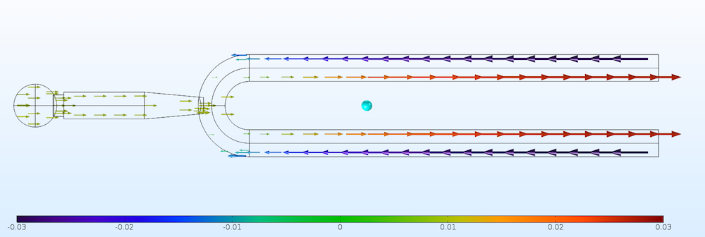
Axial displacements only. Note that the scales differ between figures. The center of gravity is indicated by the blue sphere.
Now, let’s turn to the sound emission. By adding a boundary element representation of the acoustic field to the model, the sound pressure level in the surrounding air can be computed. The amplitude of the vibration at the prong tips is set to 1 mm. This is approximately the maximum feasible value if the tuning fork is not to be overloaded from a stress point of view.
As can be seen in the figure below, the intensity of the sound decreases rather fast with the distance from the tuning fork, and also has a large degree of directionality. Actually, if you turn a tuning fork around its axis beside your ear, the near-silence in the 45-degree directions is striking.
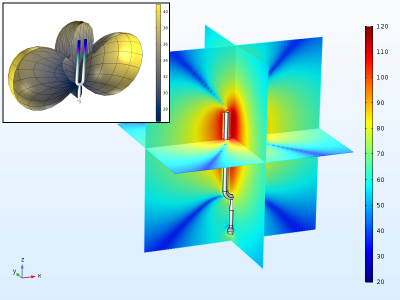
Sound pressure level (dB) and radiation pattern (inset) around the tuning fork.
We now add a 2-cm-thick wooden table surface to the model. It measures 1 by 1 m and is supported at the corners. The stem of the tuning fork is in contact with a point at the center of the table. As can be seen below, the sound pressure levels are quite significant in a large portion of the air domain above and outside the table.
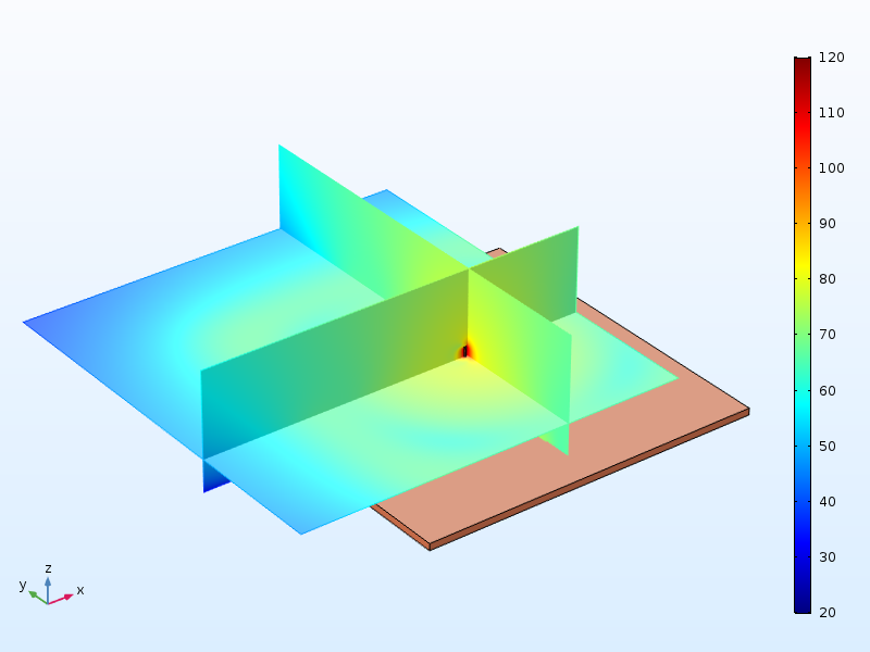
Sound pressure levels above the table when the stem of the tuning fork is attached to the table.
For comparison, we plot the sound pressure level for the same air domain when the tuning fork is held up. The difference is quite stunning with very low sound pressure levels in all parts of the air above the table except for in the vicinity of the tuning fork. This matches our experience with tuning forks as shown in the original YouTube video.
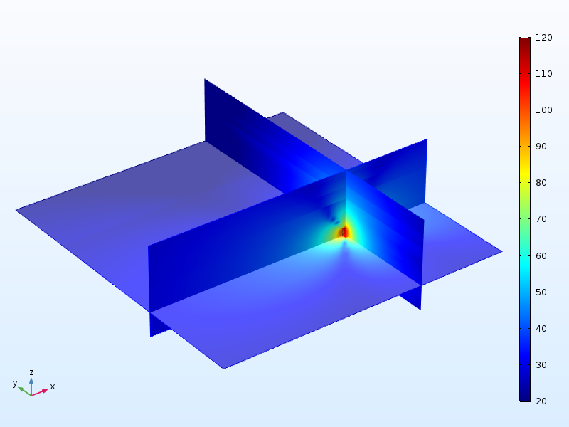
Sound pressure levels for the tuning fork when held up.
Is the Double Frequency a Natural Frequency?
So far, we have not touched on the original question: Why does the frequency double when the tuning fork is placed on the table? One possible explanation could be that there is such a natural frequency, which has a motion that is more prominent in the vertical direction. For a vibrating string, for example, the natural frequencies are integer multiples of the fundamental frequency.
This is not the case for a tuning fork. If the prongs are approximated as cantilever beams in bending, the lowest natural frequency is given by the expression
The quantities in this expression are:
- Length of the prong, L
- Young’s modulus, E; usually around 200 GPa for steel
- Mass density, ρ; approximately 7800 kg/m3
- Area moment of inertia of the prong cross section, I
- Cross-sectional area of the prong, A
For our tuning fork, this evaluates to 435 Hz, so the formula provides a good approximation.
The second natural frequency of a cantilever beam is
This frequency is a factor 6.27 higher than the fundamental frequency. It cannot be involved in the frequency doubling. However, there are other mode shapes besides those with symmetric bending. Could one of them be involved in the frequency doubling?
This is unlikely for two reasons. The first reason is that the frequency doubling phenomenon can be observed for tuning forks with different geometries, and it would be too much of a coincidence if all of them have an eigenmode with exactly twice the fundamental natural frequency. The second reason is that nonsymmetrical eigenmodes have a significant transverse displacement at the stem, where the tuning fork is clenched. Such eigenmodes will thus be strongly damped by your hand, and have an insignificant amplitude. One such mode, with a natural frequency of 1242 Hz, is shown in the animation below.
The tuning fork’s first eigenmode at 440 Hz, an out-of-plane mode with an eigenfrequency of 1242 Hz, and the second bending mode with an eigenfrequency of 2774 Hz.
The Probable Cause of the Tuning Fork Mystery
Let’s summarize what we know about the frequency-doubling phenomenon. Since it is only experienced when we press the tuning fork to the table, the double frequency vibration has a strong axial motion in the stem. Also, we can see from a spectrum analyzer (you can download such an app on a smartphone) that the level of vibration at the double frequency decays relatively quickly. There is a transition back to the fundamental frequency as the dominant one.
The dependency on the amplitude suggests a nonlinear phenomenon. The axial movement of the stem indicates that the stem compensates for a change in the location of the center of mass of the prongs.
Without going into details with the math, it can be shown that for the bending cantilever, the center of mass shifts down by a distance relative to the original length L, which is
Here, a is the transverse motion at the tip and the coefficient β ≈ 0.2.
The important observation is that the vertical movement of the center of mass is proportional to the square of the vibration amplitude. Also, the center of mass will be at its lowest position twice per cycle (both when the prong bends inward and when it bends outward), thus the double frequency.
With a = 1 mm and a prong length of L = 80 mm, the maximum shift in the position of the center of mass of the prongs can be estimated to
The stem has a significantly smaller mass than the prongs, so it has to move even more for the total center of gravity to maintain its position. The stem displacement amplitude can thus be estimated to 0.005 mm. This should be seen in relation to what we know from the numerical experiments above. The linear (440 Hz) part of the axial motion is of the order of a/100; in this example, 0.01 mm.
In reality, the tuning fork is a more complex system than a pure cantilever beam, and the connection region between the stem and the prongs will affect the results. For the tuning fork analyzed here, the second-order displacements are actually less than half of the back-of-the-envelope predicted 0.005 mm.
Still, the axial displacement caused by the second-order moving mass effect is significant. Furthermore, when it comes to emitting sound, it is the velocity, not the displacement, that is important. So, if displacement amplitudes are equal at 440 Hz and 880 Hz, the velocity at the double frequency is twice that at the fundamental frequency.
Since the amplitude of the axial vibration at 440 Hz is proportional to the prong amplitude a, and the amplitude of the 880-Hz vibration is proportional to a2, it is necessary that we strike the tuning fork hard enough to experience the frequency-doubling effect. As the vibration decays, the relative importance of the nonlinear term decreases. This is clearly seen on the spectrum analyzer.
The behavior can be investigated in detail by performing a geometrically nonlinear transient dynamic analysis. The tuning fork is set in motion by a symmetric impulse applied horizontally on the prongs, and is then left free to vibrate. It can be seen that the horizontal prong displacement is almost sinusoidal at 440 Hz, while the stem moves up and down in a clearly nonlinear manner. The stem displacement is highly nonsymmetrical, since the 440 Hz contribution is synchronous with the prong displacement, while the 880-Hz term always gives an additional upward displacement.
Due to the nonlinearity of the system, the vibration is not completely periodic. Even the prong displacement amplitude can vary from one cycle to another.
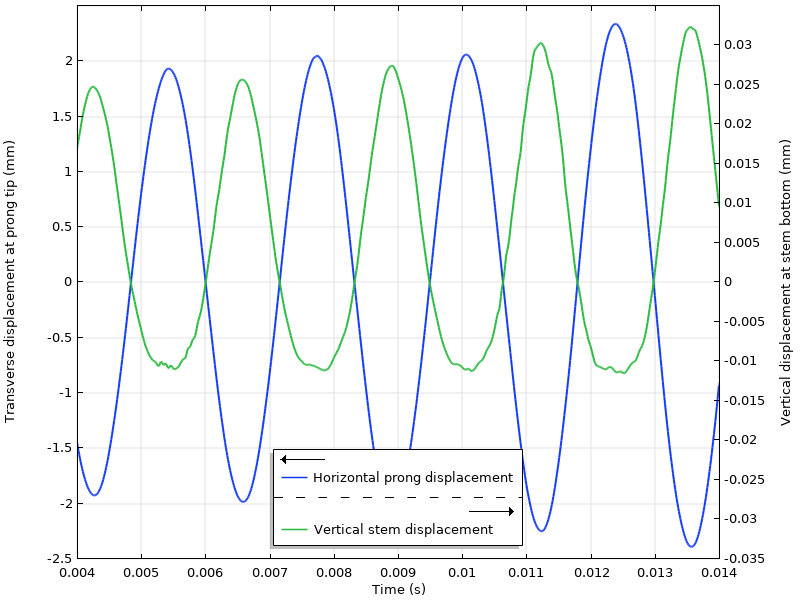
The blue line shows the transverse displacement at the prong tip, and the green line shows the vertical displacement at the bottom of the stem.
If the frequency spectrum of the stem displacement plotted above is computed using FFT, there are two significant peaks at 440 Hz and 880 Hz. There is also a small third peak around the second bending mode.
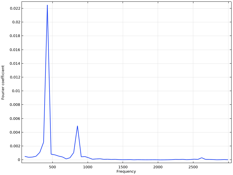
Frequency spectrum of the vertical stem displacement.
To actually see the second-order term at 880 Hz in action, we can subtract the part of the stem vibration that is in phase with the prong bending from the total stem displacement. This displacement difference is seen in the graph below as the red curve.
The total axial stem displacement (blue), the prong bending proportional stem displacement (dashed green), and the remaining second-order displacement (red).
How did we perform this calculation? Well, we know from the eigenfrequency analysis that the amplitude of the axial stem vibration is about 1% of the transverse prong displacement (actually 0.92%). In the graph above, the dashed green curve is 0.0092 times the current displacement of the prong tip (not shown in the graph). This curve can be considered as showing the linear 440 Hz term — a more or less pure sine wave. That value is then subtracted from the total stem displacement, and what is left is the red curve. The second-order displacement is zero when the prong is straight, and peaks both when the prong has its maximum inward bending and when it has its maximum outward bending.
Actually, the red curve looks very much like it is having a time variation proportional to sin2(ωt). It should, since that displacement, according to the analysis above, is proportional to the square of the prong displacement. Using a well-known trigonometric identity, \sin^2(\omega t) = \dfrac{1-\cos(2 \omega t)}{2}. Enter the double frequency!
Different Tuning Forks
Commenters on the original video from standupmaths have noticed that some tuning forks work better than others, and with some tuning forks, it is difficult to see the frequency doubling at all. As discussed above, the first criterion is that you hit it hard enough in order to get into the nonlinear regime. But there are also geometrical differences influencing the ratio between the amplitude of the two types of vibration.
For instance, prongs that are heavy relative to the stem will cause large double-frequency displacements, since the stem must move more in order to maintain the center of gravity. Slender prongs can have a larger amplitude–length (a/L) ratio, thus increasing the nonlinear term.
The design of the region where the prongs meet the stem is important. If it is stiff, then the amplitude of the fundamental frequency vibration in the stem will be reduced, and the relative importance of the double-frequency vibration is larger.
The cross section of the prongs will also have an influence. If we return to the expression for the natural frequency
it can be seen that the moment of inertia of the cross section plays a role. A prong with a square cross section with side d has
while a prong with a circular cross section with diameter d has
Thus, for two tuning forks that look the same when viewed from the side, the one with a square profile must have prongs that are a factor 1.14 longer to give the same fundamental frequency. If we assume the same maximum stress due to bending in the two tuning forks, the one with the square profile can have a transverse displacement amplitude, which is 1.142 larger than the circular one because of its higher load-carrying capacity. In addition, if the stem is kept at a fixed size, then it will become proportionally lighter when compared to the longer prongs. All these contributions end up in a 70% increase in vertical stem vibration amplitude when moving from a circular profile to a square profile.
In addition, tuning forks with a circular cross section usually have a design that is more flexible at the connection between the prongs and the stem, and thus a higher level of vibration at the fundamental frequency.
The conclusion is that a tuning fork with a square cross section is more likely to exhibit the frequency-doubling behavior than one with a circular cross section.
Do We Hear the Frequency Doubling?
In most cases, the answer is “no.” The fundamental frequency is still there, even though it may have a lower amplitude than the one with the double frequency. But the way our senses work, we hear the fundamental frequency, although with a different timbre. It is difficult, but not impossible, to strike the tuning fork so hard that the sound level of the double frequency is significantly dominant.
Conclusions
The frequency doubling occurs due to a nonlinear phenomenon, where the stem of the tuning fork must move upward, in order to compensate for the small lowering of the center of mass of the prongs as they approach the outermost positions of their bending motion.
Note that it is not the fact that the tuning fork is connected to the table that causes the frequency doubling. The reason that we measure it in that case is that the sound emitted by the resonating table surface is caused by the axial stem motion, whereas the sound we hear from the tuning fork that is held up is dominated by the prong bending. The motion is the same in both cases, as long as the impedance of the table is ignored. In fact, you can measure the doubled frequency with a tuning fork when held up as well, but it is 30 dB or so below the fundamental frequency.
Next Steps
- Watch the original videos from standupmaths on YouTube:
- Read more about the intersection of tuning forks and simulation on the COMSOL Blog:

Comments (11)
T Fernandes
April 15, 2018“Science enthusiasts” is a little bit pejorative for my taste. But it’s good to know that Comsol is approaching trending topics to appeal to a broader audience.
Ivar KJELBERG
April 15, 2018Hello Henrik
Thanks for a nice blog, showing us some of the subtleties of vibrations and resonances. By the way, in your video, you might just see that the prong is moving up and down for the higher order mode.
You know, tuning forks are not only used for a pure sound reference, they have been – and are used – in mechanical and electrical wrist watches, starting already by C. Breguet and his patent back in 1866, or to the more recent electronically driven Accutron(r) from Bulowa Swiss SA in 1960.
Today, many new patents are coming out, as with Silicon mechanics and MEMS technology one can make parts with very special shapes, so quite some work is going into new resonant escape mechanisms. But here too the mode selection is the most critical part, how to get the mechanical resonator to obey only one given mode and to damp or suppress all the others ? The answer is by playing with the shapes, or adding some other materials. Quite a program to optimize, where simulations with COMSOL Multiphysics(r) helps a lot, as no other tools allows us to mix in so many physics, to consider mixing linear but anisotropic crystals and highly non linear materials and then add easily the thermal behavior on-top.
So thanks for continuing to add improved features to the Structural Physics module, including easier and advanced mixing of other physics, it’s a great help for us to better understand our complex mechanisms, and to invent new ones.
Sincerely
Ivar
Henrik Sönnerlind
April 16, 2018Hi Mr. Fernandes,
Thank you for your comment. There was no intent to be pejorative. The standupmaths YouTube channel is qualified science presented by people who are simply enthusiastic about their topics.
Regards,
Henrik
Punnag Chatterjee
August 21, 2018Thanks so much for the detailed study of the tuning fork. Never thought about the double frequency coming from the sin^2 term.
Is it possible to get/access the COMSOL simulation file for this example?
Henrik Sönnerlind
August 23, 2018Hi Punnag,
Unfortunately, the files for these examples are not available at the moment. If they become available at a later point, we will update this post with a link to the files.
Regards,
Henrik
Joep Van Roosmalen
February 23, 2019440Hz resonates with the mind-(control)/body.
432Hz is in harmony with the spirit which is sentient energy. That’s what gives you goosebumps. It’s recognition.
Jos Groot
April 10, 2023I read: “All these contributions end up in a 70% increase in vertical stem vibration amplitude when moving from a circular profile to a square profile.” When the stem is held against a table, the circular profile has (ideally) a contact >pointsquare<. Does this point-square difference make the loudness of the sound coming from the table even higher in case of the square profile? The YouTube videos demonstrate this.
Henrik Sönnerlind
April 11, 2023 COMSOL EmployeeHi Jos,
I don’t think that the shape of the end of the tuning fork in itself affects the response of the table. From the point of view of the table, it is essentially a point excitation anyway. There is another effect that may have to be considered, though. The mass may not be the same for two different tuning forks. That would probably affect the capacity to transfer vibration to the table.
In my comparison between the circular and the square tuning fork, I assumed that they have the same projection when seen from the side. But the ‘square’ tuning fork could actually also be rectangular in profile.
Also, you can find tuning forks in both steel and aluminum in a shop, which of course would change the mass fundamentally. Interestingly enough, that choice of material does not change the size of the tuning fork, since the ratio between Young’s modulus and mass density is the same for steel and aluminum. So there are many other parameters that can obscure the conclusions.
Regards,
Henrik
Jos Groot
May 8, 2023Dear Henrik,
Thanks for your answer.
I have a question, if I may. Above is written: ‘Since the amplitude of the axial vibration at 440 Hz is proportional to the prong amplitude a, and the amplitude of the 880-Hz vibration is proportional to a², […]’. I understand where the a² for 880 Hz comes from, not where the a-dependence for 440 Hz comes from.
I myself did a simple experiment with a tuning fork very similar to the one here. The three lowest frequencies are around 440, 880 and 2750 Hz.
I held the stem between my fingers (so it was not pushed onto a resonator), and I did not hit it very hard (but what is hard?). So the 880 Hz was present even when the longitudinal stem movement was unimportant.
I also wonder what the time varying shape of the tuning fork at 880 Hz is. I could not find this on the internet.
Thanks in advance,
Jos Groot
Henrik Sönnerlind
May 9, 2023 COMSOL EmployeeHi Jos,
The 440 Hz motion is dominated by the sideways movement of the prongs. When they move outwards, then there will also be a tendency to pull the stem somewhat upwards, and when the prongs bend inwards, the stem is pushed down again. This is the 440 Hz (or first order) displacement. The reason is that the bending moment in the prongs cause bending also in the semicircular region that joins the prongs. Think about what would happen in a very wide tuning fork.
On top of that, the bending of the prongs will move their center of mass downwards, irrespective of the direction of bending. This is a cause of the second order (880 Hz) stem displacement. It is the second order effect that is quadratic in the amplitude.
The vertical motion will emit some sound even if the tuning fork is handheld, but with a different radiation pattern than the 440 Hz signal. I would guess that it is possible to pick it up better if you measure at some point above the tuning fork. However, a table is useful for amplification of the vertical movement. Even the 440 Hz signal emitted from the table comes from vertical stem motion.
When we did the experiment, using a simple cell phone app as spectrum analyzer, the decay rate of the 880 Hz signal was fairly large, indicating its quadratic dependency on the amplitude.
The 2750 Hz tone is almost certainly the second bending mode (computed to 2774 in the blog post).
The time varying shape of the fork will look no different from an animation of the first eigenmode. The second order effects are small.
Jos Groot
May 13, 2023Hi Henrik,
Thanks for your answer again. I now understand the origin of the first- and second order displacements. However, I still have one thing I do not understand.
In my measurement I see the 880 Hz (and for a short time the 3×440= 1320 Hz) harmonic component clearly in the spectrogram. I held the tuning fork in my hand, the stem was not held against e.g. a table top. Can the 880 and 1320 Hz be due to the vertical stem movement only? After all, the sound would be due the bottom of the stem and the tops of the prongs, which is together a small vibrating area. Much smaller than the tuning fork area.
On the other hand, the wavelength is much larger than this vibrating area, so the radiation pattern will be broad. As is visible in your plot entitled ‘Sound pressure level (dB) and radiation pattern (inset) around the tuning fork.’ Would it be possible to compute such a plot for the separate frequencies, i.e., for 440, 880, 1320 and 2750 Hz?
I did a quick measurement at the side and the top of the 880 Hz component (switching quickly between the two positions by rotating the tuning fork), but could not find a difference.