

Electrodynamic magnetic levitation can occur when there are time-varying magnetic fields in the vicinity of a conductive material. In this blog post, we will demonstrate how to model this principle with two examples: a TEAM benchmark problem of an electrodynamic levitation device and an electrodynamic wheel.
What Is Electrodynamic Magnetic Levitation?
Electrodynamic magnetic levitation takes place when a rotating and/or moving permanent magnet or a current-carrying coil generates a time-varying magnetic field in a nearby conductor. The time-varying magnetic fields induce eddy currents in the conductor, which create an opposing field. This in turn gives rise to a repulsive force between the conductive material and the magnetic source. This process is the fundamental operating principle of all magnetic levitation systems.
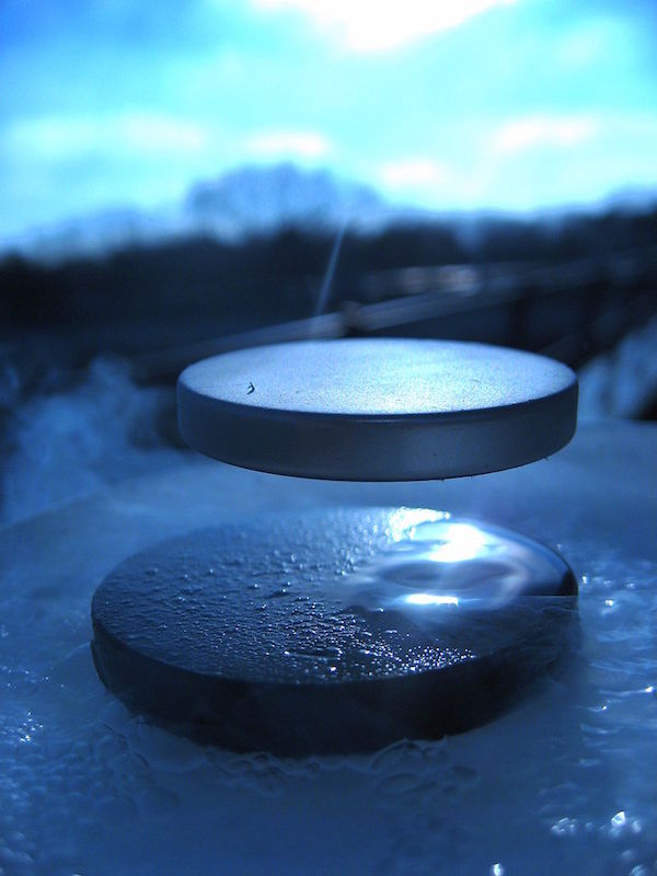
A magnet levitating above a superconductor. Image by Julien Bobroff — Own work. Licensed under CC BY-SA 3.0, via Wikimedia Commons.
Analyzing an Electrodynamic Levitation Benchmark Problem
Let’s take a look at a benchmark model based on Transient Electromagnetic Analysis Methods (TEAM) problem 28: An Electromagnetic Levitation Device. This problem consists of a circular aluminum-conducting disc placed above two cylindrical, concentric coils carrying sinusoidal currents in opposite directions. The cross-sectional cut of the setup and the dimensions are shown in the image below.
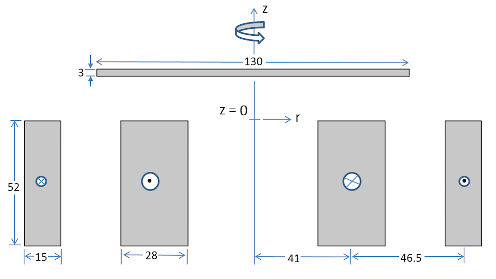
A cross-sectional view of concentric coils and an aluminum disc. All of the dimensions are in millimeters.
The model is shown in 3D below.
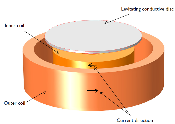
A 3D model of the electrodynamic levitation device, showing the levitated disc and two concentric coils carrying time-varying currents in opposite directions.
To model this device in the COMSOL Multiphysics® software, we use a 2D axisymmetric geometry. Due to the time-varying currents as well as the induced eddy currents, we model the magnetic fields using the Magnetic Fields interface in the AC/DC Module. The opposite current-carrying coils are modeled using separate Coil features with the Homogenized Multi-Turn Coil model. The electrodynamic force is computed in the aluminum plate by using the Force Calculation feature, which calculates the Maxwell stress tensor in it.
The rigid body dynamics of the plate are solved as a system of ordinary differential equations (ODE) via the Global ODEs and DAEs interface. The first-order ODEs for position and velocity are given by:
Since the electromagnetic force dynamically varies with distance between the plate and the coil, it is necessary to solve the Magnetic Field interface for the dynamical change in plate position. Therefore, we model the movement of the plate using the Moving Mesh interface. We compare the simulation results and the TEAM benchmark data for the corresponding position of the oscillating disc in the following plot.
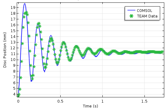
Comparing simulation results and TEAM data of the vertical plate oscillation as a function of time.
Animation depicting the oscillation of the conductive disc above the two concentric coils for 0.6 seconds.
Modeling an Electrodynamic Wheel Device in COMSOL Multiphysics®
The mechanical rotation of a magnetic source, such as a radially magnetized Halbach rotor, induces eddy currents above a passive conductive guideway (e.g., aluminum). This creates an opposing magnetic field that interacts with the source magnetic field to produce both lift and thrust forces simultaneously. This device is called an electrodynamic wheel (EDW).
The concept of EDW levitation for high-speed transportation is illustrated in the following figure. The production of the thrust or braking force depends on the relative slip speed, sl, defined as the difference between the circumferential speed, vc, and the translational speed, vx. For instance, sl = vc — vx, where vc = ωmro and ωm = ωeP. Here, ωm is the mechanical angular speed, ωe is the electrical angular speed, and P is the number of pole pairs in the Halbach rotor.
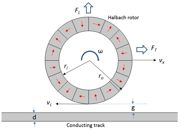
The conceptual design of a four-pole-pair EDW maglev, depicting the conductive track and rotating and/or traveling Halbach rotor.
If the circumferential speed is greater than the translational speed (for positive slip), a thrust force is generated. If the opposite is true, there will be a braking force.
Using the Rotating Machinery in 2D and 3D, Magnetic interface, we can incorporate both the translational and rotational motion in the same model. The rotational motion is specified using a Prescribed Rotational Velocity feature. The translational motion of the maglev (Halbach rotor) is accounted for in the conducting track using the Velocity (Lorentz) term with the opposite sign. The permanent magnets are modeled using the default Ampère’s Law features with remanent flux density Br = 1.42[T]. Since the magnetization direction is radial or azimuthal, we choose the cylindrical coordinate system for convenience.
The transient simulation is performed for a step change in the mechanical angular speed of the rotor. The results for the lift and thrust forces as a function of time are shown below. These forces are calculated by two different methods: the Maxwell stress tensor (using the Force Calculation feature) and the Lorentz method.


The comparison of lift and thrust forces on the maglev as a function of time. Results from both the Maxwell stress tensor and Lorentz method are shown.
In the second step, the stationary simulation is performed for a range of translational speeds. A drag force is generated if there is no rotation or the circumferential speed is less than the translational speed. The simulation results for the lift and drag forces for various speeds are shown below.


The comparison of lift and drag forces on the maglev as a function of velocity. Results from both the Maxwell stress tensor and Lorentz method are shown.
Animation depicting the surface plot of the magnetic flux density in the air and magnets; current density in the guideway; and the contour plot of magnetic vector potential, Az. The clockwise rotation of the Halbach rotor and the field interactions are shown.
Summary on Modeling Electrodynamic Magnetic Levitation
In today’s blog post, we demonstrated how to model two electrodynamic magnetic levitation devices using COMSOL Multiphysics and the add-on AD/DC Module. We featured TEAM problem 28: Electrodynamic Levitation Device and compared the results with experimental data from literature. We also highlighted the working principle of an electrodynamic wheel magnetic levitation system. Our simulation results show the lift and drag/thrust forces generated by this system for a step change in the angular speed and various translational velocities.
Further Reading
- Learn more about the examples featured in this blog post:
- See how others have used COMSOL Multiphysics to solve similar magnetic levitation systems
- Browse other blog posts featured in our Electromagnetic Device series
- Want to start modeling magnetic levitation systems in COMSOL Multiphysics or have additional questions on your current modeling processes? Contact us


Comments (2)
Ivar Kjelberg
November 30, 2016A beautiful illustration of the force of COMSOL, as teaching tool, to really understand the physical phenomena, one can later add thermal dissipation, heating resistance heat dependence, and see these secondary effects, then aerodynamic drag forces, and so on.
Just a pity that so many institutions do not use COMSOL more efficiently: lets try to change that!
It’s my objective, to start in 2018.
Trevor Munroe
December 5, 2016As usual, Nirmal’s blogs is always very good (so also many of the other blogs). I agree with the above comment. So much more can be done. I modified the model provided in the blog by taking out the plate dynamic equations and using the Structural Module instead with gravity turn-on. It ran just fine.